A collective tracking method for preliminary
sperm analysis
Sung‑Yang Wei
1, Hsuan‑Hao Chao
1, Han‑Ping Huang
1, Chang Francis Hsu
1, Sheng‑Hsiang Li
2,3*and Long Hsu
1*Abstract
Background: Total motile sperm count (TMSC) and curvilinear velocity (VCL) are two important parameters in preliminary semen analysis for male infertility. Traditionally, both parameters are evaluated manually by embryologists or automatically using an expensive computer‑assisted sperm analysis (CASA) instrument. The latter applies a point‑tracking method using an image processing technique to detect, recognize and classify each of the target objects, individually, which is complicated. However, as semen is dense, manual counting is exhausting while CASA suffers from severe over‑ lapping and heavy computation.
Methods: We proposed a simple frame‑differencing method that tracks motile sperms collectively and treats their overlapping with a statistical occupation probability without heavy computation. The proposed method leads to an overall image of all of the differential footprint trajectories (DFTs) of all motile sperms and thus the overall area of the DFTs in a real‑time manner. Accordingly, a theoretical DFT model was also developed to formulate the overall DFT area of a group of moving beads as a function of time as well as the total number and average speed of the beads. Then, using the least square fitting method, we obtained the optimal values of the TMSC and the aver‑ age VCL that yielded the best fit for the theoretical DFT area to the measured DFT area. Results: The proposed method was used to evaluate the TMSC and the VCL of 20 semen samples. The maximum TMSC evaluated using the method is more than 980 sperms per video frame. The Pearson correlation coefficient (PCC) between the two series of TMSC obtained using the method and the CASA instrument is 0.946. The PCC between the two series of VCL obtained using the method and CASA is 0.771. As a con‑ sequence, the proposed method is as accurate as the CASA method in TMSC and VCL evaluations.
Conclusion: In comparison with the individual point‑tracking techniques, the col‑ lective DFT tracking method is relatively simple in computation without complicated image processing. Therefore, incorporating the proposed method into a cell phone equipped with a microscopic lens can facilitate the design of a simple sperm analyzer for clinical or household use without advance dilution.
Keywords: Object tracking, Frame differencing, Computer‑assisted sperm analyzer (CASA), Total motile sperm count (TMSC), Curvilinear velocity (VCL)
Open Access
© The Author(s) 2019. This article is distributed under the terms of the Creative Commons Attribution 4.0 International License (http://creat iveco mmons .org/licen ses/by/4.0/), which permits unrestricted use, distribution, and reproduction in any medium, provided you give appropriate credit to the original author(s) and the source, provide a link to the Creative Commons license, and indicate if changes were made. The Creative Commons Public Domain Dedication waiver (http://creativecommons.org/publicdo‑ main/zero/1.0/) applies to the data made available in this article, unless otherwise stated.
RESEARCH
*Correspondence: [email protected]; [email protected] 1 Department
Background
Semen analysis is essential in both clinical and research settings for investigating male fertility status, which affects approximately 15% of couples throughout the USA [1]. A normal sperm concentration of semen ranges from 15×106 to 259×106/ml
[2]. Healthy sperms are motile in semen. Excessive immotile sperms result in male infertility. The total sperm count (TSC) and the motility, the ratio of the total motile sperm count (TMSC) to the TSC within a same volume [3], are important parameters for measuring sperm fertility.
According to the latest (2010) World Health Organization (WHO) standard for nor-mal sperm [3], the minimal concentration and motility of total sperms have been low-ered to 15.0×10⁶/ml and 40.0%, respectively [4]. The product of these two numbers,
15×106/ml
×40.0%=6×10⁶/ml
, indicates the minimal concentration of total motile sperms for normal sperm because motility is equivalently the ratio of the con-centration of total motile sperms to the concon-centration of total sperms of a semen [3].
Some researchers have reported that the TMSC shows a better correlation with the spontaneous ongoing pregnancy rate than the WHO 2010 classification system [5,
6]. Consequently, the TMSC [7, 8] and the curvilinear velocity (VCL) [9–11] of the motile sperms are two of the characteristic parameters of a semen sample in a pre-liminary semen analysis as well. Note that the VCL is the average speed of a sperm head through its real path.
Traditionally, dozens of individual sperm parameters can be evaluated using an automatic computer-assisted sperm analysis (CASA) instrument [12, 13] that tracks the trajectory of every sperm individually using a point-based tracking technique [14]. However, the individual point-tracking technique requires heavy computation for complicated image processing to detect, recognize and classify each of the target objects, individually [15]. As a semen sample is dense, severe overlapping of sperms would degrade the accuracy of CASA [16, 17]. The disadvantages make the CASA instrument expensive for clinical use and subject to semen concentration below 50×106/ml , as suggested by the WHO 2010 standard [3]. In other words, a semen sample of higher concentration requires advance dilution. However, not only is dilu-tion inconvenient to the users but every diludilu-tion also increases the inaccuracy of the measurement. Recently, the overlapping problem inherited from the point-tracking technique has been greatly alleviated by using multi-target tracking algorithms [17–
20]. Nevertheless, the required powerful algorithms increase the computation load. As alternatives, inexpensive sperm analyzers are also now available [21–23]. These commercial products can analyze dense semen samples without advance dilution. However, their working mechanisms do not distinguish the motile sperms from the immotile or measure the speeds of the sperms.
In this paper, we proposed a collective rather than individual tracking method for esti-mating the total number and average speed of up to 980 motile sperms without using complicated image processing. Using a frame-differencing technique [28–30], the pro-posed method leads to an overall image of all of the differential footprint trajectories (DFTs) of all motile sperms and thus the overall area of the DFTs in real time. Accord-ingly, a theoretical DFT model was developed to formulate the overall DFT area as a func-tion of time as well as the total number and average velocity of a group of moving objects. In the DFT model, the problem of overlapping is treated using a statistical occupation probability. Finally, the DFT method was examined in the evaluations of TMSC and VCL using 20 semen samples and 523 synthetic bead samples. Using the least square fitting method, we obtained the optimal values of the TMSC and the average VCL that yielded the best fit for the theoretical DFT area to the measured DFT area. The results were found to be strong correlated with those obtained using manual counting and the CASA instrument used in this study, separately. Therefore, it will be shown that the proposed DFT method is simple in computation and appropriate for preliminary sperm analysis.
Results
Insignificant influence of Gaussian speed distribution on TMSC and VCL
From the results of the first type of simulation conducted using the first 400 synthetic bead samples, Table 1 shows the percentage errors
EN_DFT,Ev_DFT
between the optimal
NDFT,vave_DFT
and the preset
Nset=1000,vave_set=60µm/s for the four settings of
δset at 0, 18, 36 and 54 µm/s under the condition of Nset=1000 , separately. Note that
the simulation for each δset was conducted 100 times for the average of
NDFT,vave_DFT
. As the table shows, the maximal percentage errors of EN_DFT and Ev_DFT were 7.42% at δset=18 and 2.09% at δset=0 , respectively. As a whole, the overall averages of the per-centage errors
EN_DFT,Ev_DFT
were (7.10% and 1.79%), respectively.
DFT method as accurate as CASA in TMSC and VCL evaluations in simulation
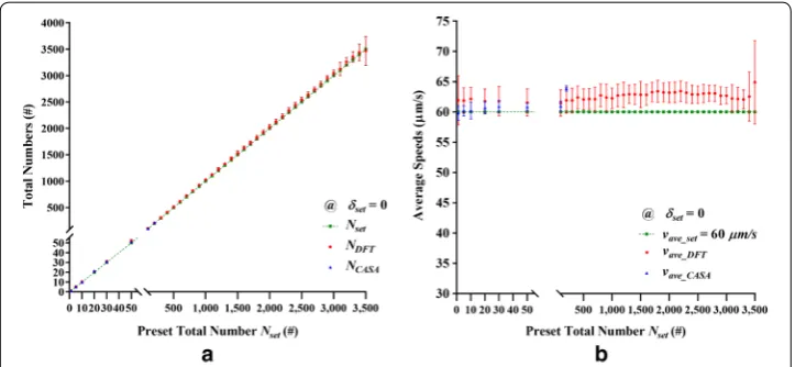
From the results of the second type of simulation conducted using the remaining 123 synthetic bead samples, Fig. 1 shows the optimal
NDFT,vave_DFT evaluated using
the DFT method, the
NCASA,vave_CASA
measured by the CASA instrument, and the
Nset,vave_set
preset for the 41 settings of Nset under the condition of vave_set=60µm/s and δset=0µm/s . Specifically, Fig. 1a shows the total numbers NDFT and NCASA versus
Table 1 Results of the first kind of simulation conducted using the first 400 synthetic bead samples: the percentage errors EN_DFT and Ev_DFT of the total number NDFT and the average speed vave_DFT of a group of synthetic beads due to their Gaussian speed distributions set at four different standard deviations δset
δset(µm/s) @ Nset=1000 vave =60µm/s
0 18 36 54 Overall average
NDFT(#) 1069.77 1074.23 1072.46 1067.35 1070.95
Standard deviation (#) 36.42 34.80 39.92 44.22 38.84
Percentage error EN_DFT(%) 6.98 7.42 7.25 6.74 7.10
vave_DFT(µm/s) 61.26 60.93 60.97 61.15 61.08
Standard deviation (µm/s) 1.32 1.26 1.46 1.61 1.41
the preset Nset that serves as the reference. It can be seen that the three series of NDFT , NCASA and Nset form a straight line. The linear correlation between any two series among
NDFT , NCASA , and Nset was measured by using the Pearson correlation coefficient (PCC)
analysis [31, 32]. The resulting PCCs were found to be greater than 0.999 with the corre-sponding P‐values less than 0.001. In principle, a P‐value less than 0.05 is considered as statistically significant [33]. This indicates that the three series obtained using the three different methods were strongly correlated with a high statistical significance. In addi-tion, the overall average percentage error EN_DFT was 2.36% in comparison with Nset.
As for the average speed, Fig. 1b shows the average speeds vave_DFT and vave_CASA ver-sus the preset vave_set=60µm/s . The overall average percentage error Ev_DFT was 4.35% in comparison with vave_set.
DFT method as accurate as CASA in TMSC and VCL evaluations in experiment
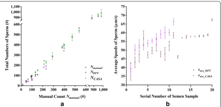
From the results of the experiment conducted using the 20 human semen sam-ples, Fig. 2 shows the optimal
NDFT,vave_DFT
evaluated using the DFT method, the
NCASA,vave_CASA
measured using the CASA instrument, and the Nmanual obtained by manual counting, separately. Specifically, Fig. 2a shows the total numbers NDFT and NCASA versus the manual count Nmanual that serves as the gold standard. It can be seen that the maximum NDFT or TMSC evaluated using the DFT method is greater than 980 sperms per video frame. In addition, the series of NDFT and NCASA are close to the series
of Nmanual . The PCC between the series of NDFT and Nmanual was found to be 0.996 with a P-value less than 0.001. While that between the series of NDFT and NCASA was found to
be 0.946 with a P-value less than 0.001. As a whole, the overall average of the percentage errors EN_DFT was 15.33% in comparison with the manual counts. Yet, the overall aver-age of the coefficient of variation (CV) of the manual counting results was 5.81%.
As for the average speed, Fig. 2b shows only the average speeds vave_DFT and vave_CASA
versus the serial number of the 20 semen samples, since it is difficult to estimate the
Fig. 1 Results of the second type of simulation conducted using the 123 synthetic bead samples at 41 settings of Nset and δset=0 . a Total numbers NDFT and NCASA versus the preset Nset ranging from 1 to 3500. b
Average speeds vave_DFT and vave_CASA versus the preset vset . Red points: NDFT and vave_DFT evaluated using the
DFT method. Blue points: NCASA and vave_CASA measured using the CASA instrument. Green points: preset Nset
speeds of sperms manually. Accordingly, the PCC between the series of vave_DFT and vave_CASA was found to be 0.771 with a P-value less than 0.006. It can be seen that, in
general, the series of vave_CASA is slightly higher than that of vave_DFT in Fig. 2b. The series of NCASA is slightly lower than that of NDFT in Fig. 2a. This tendency will be discussed in the discussion section.
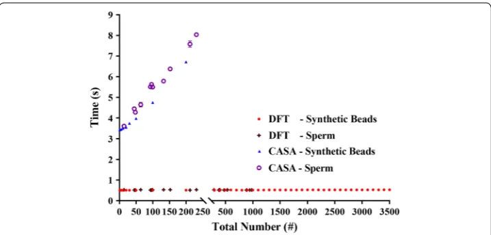
Computation times of DFT method and CASA
Figure 3 illustrates the computation times of the DFT method, using the collective track-ing technique, and the CASA method, applytrack-ing a point-tracktrack-ing technique, as a function of the total numbers of synthetic beads and sperms. It can be seen that the DFT method demonstrated a larger count range of TMSC for both synthetic beads and sperms in less time than the CASA method. In addition, the computation time of the DFT method was found independent of the number of synthetic beads or sperms while that of the CASA method increased with the total numbers of synthetic beads and sperms. This supports that the collective DFT method is effective and simple in the evaluation of the total number and average velocity of a group of moving objects.
Discussion
As shown in Table 1, the results of the first type of simulation indicated that the influ-ence of the Gaussian speed distribution of a group of beads on the evaluations of NDFT
and vave_DFT is insignificant in the DFT method. This can be explained in principle.
Referring to Fig. 5, one can imagine that the DFT area contributed by the beads that are faster than the average speed just compensates for that contributed by the beads slower than the average speed. This suggests that the DFT method is also valid for a group of beads, such as healthy semen, with a symmetric speed distribution by assuming that they move at their average speed.
Fig. 2 Results of the experiment conducted using 20 semen samples. a Total numbers NDFT and NCASA versus
the manual count Nmanual that serves as the gold standard. b Average speeds vave_DFT and vave_CASA versus
the serial number of the 20 semen samples. Green points: the manual counts Nmanual . Dark red points: NDFT
and vave_DFT evaluated using the DFT method. Violet points: NCASA and vave_CASA measured using the CASA
As shown in Fig. 1, the results of the second type of simulation exhibited separately that the accuracy of the DFT method in the evaluation of NDFT is as high as that of
the CASA instrument in comparison with the preset Nset . The resulting PCCs were all greater than 0.999 with the corresponding P‐values all less than 0.05. The over-all averages of the percentage errors EN_DFT of 2.36% and Ev_DFT of 4.35% were all less than 5.0%. This performance persisted until there were 3500 synthetic beads for which overlapping was severe. This justifies the statistical treatment of the occupation probability for the overlapping problem in the proposed DFT model.
However, as shown in Fig. 2, the experimental results evaluated using the DFT method showed a relatively high percentage error EN_DFT of 15.33% in comparison with the manual counts Nmanual . The results also showed a relatively low PCC of 0.771 with a P‐value less than 0.05, in comparison with the average speed vave_CASA
meas-ured using the CASA instrument. The deterioration of the experimental results is likely due to the following three factors:
First, a finite CV of 5.81% for the series of manual counts Nmanual existed because most semen samples had high concentrations. Second, sperms slower than the cutoff speed of 5µm/s were not counted by the CASA instrument by default. Thus, the series of vave_CASA tended to be slightly faster than that of vave_DFT , as shown in Fig. 2b. The
series of NCASA tended to be slightly less than that of NDFT, as shown in Fig. 2a. Third,
the real sperms are different from the synthetic beads in size and speed distribution. The consequence is attributed to the limitation of the DFT method. As discussed above, any asymmetry on the size or speed distribution of a semen sample would degrade the accu-racy of the DFT method since the TMSC and VCL of a semen sample are evaluated from the overall area of the DFT of all motile sperms in the sample. Therefore, removing the first two factors caused by the manual counting and the CASA instrument, separately, one might expect that the overall averages of the percentage errors EN_DFT and Ev_DFT
caused by the DFT method alone would be reduced.
Nevertheless, the two PCCs of 0.946 and 0.771 are all greater than 0.7, and the results of the DFT method and those of the CASA instrument are considered strong correlated [31, 32]. Consequently, the DFT method is as accurate as the CASA method in the evaluations of TMSC and VCL.
In this study, the unhealthy semen samples were found containing more slow sperms than fast ones. It can be imagined that a small or slow sperm contributes a smaller DFT area than a large one. The more the slow sperms, the smaller the overall DFT area and thus the less the TMSC in comparison with the manual count. The case of unhealthy semen elucidates the limitation of the DFT method on the sym-metry of the size and speed distribution of a group of target objects. In this sense, it is recommended to carry out the simple semen analysis right after a semen sample is collected to prevent the motility of the sperms from dropping too fast [34], which will change the speed distribution of the semen sample.
Conclusion
A collective DFT tracking method was proposed for evaluating the total number and average speed of a group of moving objects. In the DFT model, the objects are assumed to be identical in size. Their speeds can be either the same or different with a symmetric distribution. The proposed DFT method tracks the moving objects col-lectively and treats any overlapping using a statistical occupation probability without heavy computation. In this study, the DFT method was used to evaluate the TMSC and VCL of 523 synthetic bead samples in the simulation and 20 semen samples in the experiment. Recall that both TMSC and VCL are two characteristic parameters in preliminary sperm analysis.
The maximal count range of TMSC obtained using the DFT method is up to 980 sperms per video frame in the experiment and 3500 synthetic beads per frame in the simulation. The experimental results showed that the PCC between the two series of TMSC obtained using the DFT method and the CASA instrument was 0.946. The PCC between the two sets of VCL obtained using the method and the CASA instru-ment was 0.771. Their corresponding P-values were all less than 0.05. This indicates that the results obtained using the DFT method and those of the CASA instrument were strongly correlated with a high statistical significance [31, 32]. As a conse-quence, the proposed DFT method is as accurate as the CASA instrument in evalu-ating TMSC and VCL. This also verifies the validity of the DFT model.
In comparison with those individual point-tracking techniques, the collective DFT tracking method is relatively simple in computation without complicated image cessing and provides a large count range of TMSC. Therefore, incorporating the pro-posed method into a microscope or a cell phone equipped with a microscopic lens can facilitate the design of a simple sperm analyzer as accurate as CASA for clinical or household use without advance dilution.
In future work, the accuracy of the TMSC and VCL can be further improved by using a 4 K (3840×2160) resolution image sensor instead of the 640×480 one since
Methods
The algorithm used in the proposed collective tracking method is simple. Consider a 10-s-long video film recorded with the charge-coupled device (CCD) camera inside the CASA instrument used in this study. First, two consecutive video frames of a semen sample were subtracted pixel by pixel. A unique color was marked on those resulting pixels whose absolute values are above a given threshold value. The resulting image shows the footprints of all motile sperms in a differential manner. Then, the subtrac-tion process was repeated over a series of frames and the resulting differential footprint images were superimposed one after the other. This results in an overall image of the entire DFTs of all motile sperms.
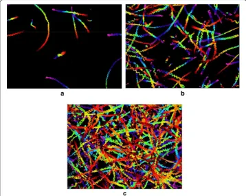
Color‑coded DFT
Figure 4 illustrates the typical color-coded DFT images of three semen samples of dif-ferent concentrations for 10 s, individually. Each trajectory in the images represents a motile sperm. The longer and more colorful a trajectory is, the faster the correspond-ing sperm moves. As time goes by, each DFT extends and the overall area of the DFT increases with time.
In the following sections, the concept, model and procedure of the DFT method will be presented. The dependence of the overall DFT area on the total number and aver-age speed of the moving objects is illustrated. An equation of the overall DFT area as a
Fig. 4 Typical color‑coded DFT images of three semen samples of different concentrations for 10 s under a
function of time as well as the total number and average velocity of a group of moving objects is developed. The optimal values of the total number and average speed of the moving objects can be derived using the least square fitting method. Subsequently, 20 semen samples and 523 synthetic bead samples were prepared and recorded into gray-scale instead of color-coded videos for the test of the proposed DFT method in the eval-uations of TMSC and VCL. The test process was conducted by comparing the results evaluated using the DFT method with those obtained using the manual count method and the CASA instrument used in the study.
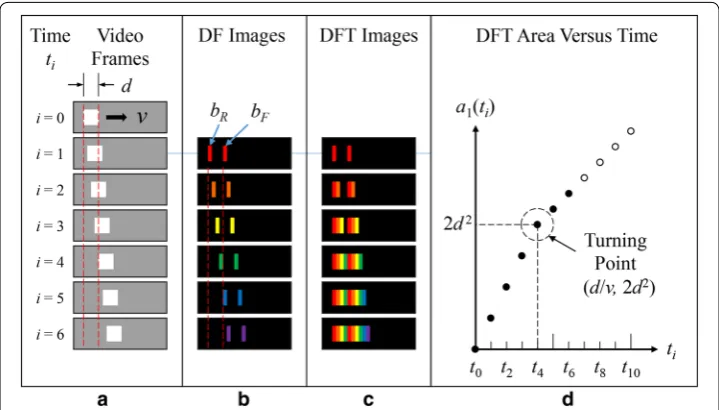
Concept: one‑dimensional DFT of a single moving square
For simplicity, we first considered a square of width d moving at a constant speed v in one dimension. Figure 5a shows the continuous displacement of the square in seven consecutive video frames during a period from t0=0 to t6=6t . Herein, ti=it.
where i is an integer representing the frame number and t is a unit time interval. In
this case, d=4vt is assumed such that the square moves a distance of a body length
d at t4=4t . Figure 5b shows a series of six differential footprint images of the square
in different colors. Each image displays a rear and a front rectangle. This is obtained by subtracting two consecutive frames and coding the resulting frame with a unique color for the pixels whose absolute values are above a given threshold value. Each pair of rec-tangles is called the differential footprint of the square from a single move.
Figure 5c illustrates the growth of the color-coded DFT of the moving square as a function of time by superimposing the six differential footprint images in succession. Notice that only the first four footprints appear in pairs in Fig. 5c. Subsequently, only the front rectangle of each succeeding pair appears in the DFT since the rear one always overlaps the front of a previous pair. The peculiar feature of the DFT method is reflected in Fig. 5d, a plot of the area of the DFT as a function of time. It can be seen that the DFT
area a1(ti) increases with time ti at two slopes separated at a turning point. This feature
can be expressed using the following equation for a1(ti):
where the subscript “1” indicates a single square, i is the video frame number, and bR as
well as bF are the areas of the rear as well as the front rectangles of a differential
foot-print, respectively. Under the condition bR=bF=dvt , the coordinates of the turning
point are
d/v, 2d2
. In other words, the turning point reflects the speed v of the moving square.
Model: two‑dimensional DFT of a group of moving beads
To be realistic, we further considered a group of identical beads with each of diameter d moving randomly at the same speed v in two dimensions. Initially, the locations and directions of movement of the beads are randomly distributed over a video frame. Fig-ure 6 illustrates the concept of the DFT method used in developing the equation of the overall DFT area A3(t1) of three beads from two consecutive video frames at t0 and t1 in the presence of bead overlapping. As shown in Fig. 6, each pair of crescents in red is the differential footprint of a bead. The overlapping of the three footprints changes the effective footprint area of each bead. The idea of evaluating the overall footprint area of the three beads at t1 is to add the effective footprint area of each bead successively as fol-lows. First, Fig. 6a shows the differential footprint of a single bead from a move. Regard-less of the direction of the movement of the bead, the corresponding DFT area A1(t1) of
the bead is given by A1(t1)=BR+BF , where BR and BF are the areas of the rear and the front crescents, respectively. Here, the symbols A1 , BR and BF are rewritten in upper case in the model of multiple beads. Note that BF(=dv�t) remains constant at all times whereas BR can be approximated to be the average area of the various rear crescents such that BR=BR(ti)=
π 4
dv�t.
Second, Fig. 6b shows a statistical treatment of the overlapping of two beads. In the presence of a second bead anywhere in the frame, the probability for the second bead to
(1)
a1(ti)=
i(bR+bF) fori≤ v�td
d
v�t(bR+bF)+ �
i− v�td �bF fori> v�td ,
occupy a full differential footprint of the area (BR+BF) depends on the percentage of the
empty area over the full area of the video frame from a statistical point of view. Accord-ingly, the occupation probability for a bead to occupy a full differential footprint is defined as
1−Aoccupied/C
, where C is the full area of the video frame and Aoccupied is the area that has been occupied. In this case, the occupied area Aoccupied is A1(t1) and A1(t1)/C is
the percentage of the occupied area over the frame. The resulting occupation probability is [1−A1(t1)/C] . Thus, the effective area occupied by the differential footprint of the second
bead becomes (BR+BF)[1−A1(t1)/C] , which is the product of the full area (BR+BF) and
the occupation probability. Statistically, the overall DFT area A2(t1) of the two beads is the sum of the two effective areas of the first and the second beads, as given by:
Third, Fig. 6c shows a simple geometric progression formula for the overlapping of three beads. Similarly to the statistical treatment of two beads, the presence of the third bead creates an additional effective area (BR+BF)[1−A2(t1)/C] . Thus, the overall DFT area A3(t1) of the three beads can be expressed as:
It is worth noting that A3(t1) is in the form of a geometric series and thus can be expressed in compact form as A3(t1)=C1−[1−(BR+BF)/C]3 . Further, the overall DFT area AN(t1) of N beads at t1 can be expressed as
Based on the same idea, for the succeeding video frame at time t2 , the overall DFT area AN(t2) of the same number N of beads can be expressed in the form:
Similarly to the turning point for a single moving square, as shown in Eq. (1) for
a1(ti) , AN(ti) also presents a turning point for N moving beads. It can be imagined that both crescent areas BR and BF of each bead contribute to the overall DFT area before the bead moves a distance of a body length d for ti≤d/v or i≤d/(v�t) . Sub-sequently, for ti>d/v or i>d/(v�t) , only the front crescent area BF of each bead contributes to the overall DFT area. As a consequence, it can be shown that the over-all DFT area AN(ti) of N identical beads in a video frame at time ti can be expressed as Eq. (6).
(2)
A2(t1)=A1(t1)+(BR+BF)
1− A1(t1) C
=(BR+BF)
1+
1− (BR+BF)
C .
(3)
A3(t1)=A2(t1)+(BR+BF)
1−A2(t1) C
=(BR+BF)
1+
1− (BR+BF) C
+
1−(BR+BF) C
2
.
(4)
AN(t1)=C
1−
1−BR+BF
C
N
.
(5)
AN(t2)=C
1−
1−BR+BF
C
2N
Indeed, the overall DFT area AN(ti) is a function of time ti , the total number N and the average velocity v. Here, N and v serve as implicit parameters. Under the condition
(BR+BF)/C≪1 for small beads, Eq. (6) for AN(ti) can be simplified in the following form, by making use of Taylor’s expansion technique,
Notice that Eq. (6) resembles Eq. (1) as AN(ti)≈Na1(ti) when the square in Eq. (1) is replaced with a bead. The consequence of a linear relation between multiple beads and a single bead is reasonable since bead overlapping is negligible in a group of small beads that are sparsely distributed. The applicability of Eq. (7) to small beads supports the sta-tistical treatment of occupation probability for the bead overlapping problem in deriving Eq. (6) for AN(ti).
Effect of Gaussian speed distribution on TMSC and VCL
In reality, the motile sperms in a semen sample [35] move at various speeds that follow a Gaussian-like symmetric probability distribution [36]. It is to be noted that the prob-ability density of a Gaussian speed distribution is given by:
where vave is the average speed and δ is the standard deviation of the Gaussian speed dis-tribution. Thus, it is too complicated to develop further an analytic equation for the DFT area as a function of time in this case. Instead, through simulation, the overall DFT area AN(ti) versus time ti was plotted for a group of N beads whose speeds follow a Gaussian
distribution, as discussed above. For comparison, a graph of AN(ti) versus ti was also plotted for the same N beads but with all beads moving at the same average speed vave of the Gaussian speed distribution. The simulation results demonstrated later will show that the two plots are nearly the same. Consequently, this allows us to use Eq. (6) for AN(ti) in the analysis of real semen samples.
Procedure of DFT method
Similarly to the procedure for a single moving square as illustrated in Fig. 5, the pro-cedure of the DFT method for a target semen sample or synthetic bead sample was as follows. First, a series of 30 consecutive grayscale video frames of the target sam-ple were acquired, as shown in Fig. 5a. In this study, the resolution of the video frames was 640×480 pixels. The gray levels of the video frames ranged from 0 to 255. Second, any two consecutive frames were subtracted pixel by pixel. A new number “255” was assigned on those resulting pixels whose absolute values were above a threshold value,
(6)
AN(ti)= C �
1−�1−BR+CBF�iN �
fori≤ v�td
C �
1−�1−BR+CBF�
dN v�t
�
+C�1−BR+CBF�
dN v�t
�
1−�1−BFC� �
i−v�dt
� N�
fori> v�td .
(7)
AN(ti)=
iN(BR+BF) fori≤ v�dt
dN
v�t(BR+BF)+ �
i− v�dt�NBF fori> v�dt
.
(8)
f(v)= 1 δ√2πe
20 in this case, and a new number “0” was assigned elsewhere. This marked a differen-tial footprint image of all motile sperms or synthetic beads, as shown in Fig. 5b. Third, the subtraction process was repeated through the 30 consecutive frames in sequence and the resulting differential footprint images were superimposed in succession. This resulted in 29 images of all of the DFTs of all sperms or beads at different times, show-ing the extension of the entire DFTs as a function of time, as shown in Fig. 5c. The total number of the pixels whose values were not “0” on a DFT image at time ti was just the overall area ADFT(ti) , in pixels, of all of the DFTs on that image. Fourth, the overall DFT area of each of the 29 DFT images, ADFT(ti) for 1≤i≤29 , was calculated and plotted
versus time, as shown in Fig. 5d. Last, the least square fitting method was used to obtain the optimal values of NDFT and vave_DFT that yielded the best fit for Eq. (6) for the theo-retical ADFT(ti) to the above measured ADFT(ti).
The above image process is collective rather than individual. It does not need to recog-nize and classify each of the target objects, individually. Thus, the DFT method is simple in computation without complicated image processing.
CASA settings
The CASA instrument used in the study (IVOS CASA System manufactured by Hamil-ton-Thorne Research) was set as follows: negative phase-contrast optics and recording at the frame rate: 60 Hz; frames acquired: 30; magnification: 10× objective; minimum con-trast: 80; minimum cell size: 3 µm; non-motile head size: 5 µm; non-motile head inten-sity: 160; medium average path VCL cutoff: 25 µm/s; low path VCL cutoff: 5 µm/s; and threshold straightness: greater than 80% [37].
Manual counting
Each semen sample was counted three times for averaging by three researchers trained at Mackay Memorial Hospital Reproductive Medicine Center, New Taipei City, Taiwan. The use of semen for research had been reviewed and approved by the hospital’s institu-tional review board with the approval number 14MMHIS280.
Experiments and simulations
Twenty semen samples and 523 synthetic bead samples were used to verify the validity of the proposed DFT method in the evaluations of TMSC and VCL. In particular, two types of simulations were conducted using the 523 synthetic bead samples for two pur-poses. One was to estimate the influence of the speed distribution of a group of synthetic beads on the evaluation of the total number of beads in the proposed DFT method. The other was to evaluate the influence of the total number of beads on the accuracies of the DFT method on the evaluations of the total number and average speed of the beads.
In the first type of simulation, δset was set to 0, 18, 36 and 54 at the preset Nset=1000
and vave_set=60µm/s , separately. For each setting of δset , the optimal values of NDFT
and vave_DFT of the corresponding synthetic bead sample in a video were first evaluated
following the procedure of the DFT method. Then, the optimal
NDFT,vave_DFT
was compared with the preset (Nset=1000,vave_set=60µm/s) and the percentage errors
EN_DFT≡(NDFT−Nset)/Nset and Ev_DFT≡
vave_DFT−60
/60 were obtained,
DFT model. As a consequence, the percentage errors
EN_DFT,Ev_DFT
at various δset
reflect the influence of the speed distribution of the beads on the evaluations of NDFT
and vave_DFT in the DFT method.
In the second type of simulation, Nset was set to 41 different values ranging from 1 to 3500 at δset=0 and vave_set=60µm/s , separately. For each setting of Nset , the optimal NDFT and vave_DFT of the synthetic bead sample in a video were first evalu-ated following the procedure of the DFT method. Then, these synthetic videos were sent to the CASA instrument to measure the total number NCASA and the VCL
vave_CASA of the Nset beads for comparison. Thus, the corresponding percentage errors
EN_CASA≡(NCASA−Nset)/Nset and Ev_CASA≡
vave_CASA−60
/60 were obtained. As a consequence, the errors
EN_DFT,Ev_DFT
and
EN_CASA,Ev_CASA
reflect the accuracies of the DFT method and the CASA instrument on the evaluations of
NDFT,vave_DFT
and
NCASA,vave_CASA
, respectively.
To reduce uncertainties, every simulation of the first type was conducted 100 times for the average of
NDFT,vave_DFT
. Thus, 400 different bead samples were synthesized and analyzed for the four settings of δset at Nset=1000 and vave_set=60µm/s . In addi-tion, every simulation of the second type was conducted three times for the averages of
NDFT,vave_DFT and NCASA,vave_CASA . Thus, 123 different bead samples were syn-thesized and analyzed for the 41 settings of Nset at δset=0 and vave_set=60µm/s . In total, 523 synthetic bead samples were analyzed in the two types of simulations. On the other hand, every semen experiment was conducted three times for the averages of
NDFT,vave_DFT , NCASA,vave_CASA
, and Nmanual . Thus, the 20 different semen samples
were analyzed 60 times in total.
Sperm preparation
Twenty human semen samples were selected from 31 subjects for a wide distribution of TMSCs and VCLs of the sperms from unhealthy to healthy. The semen samples were collected by masturbation after 2 to 3 days of sexual abstinence. After liquefaction for at least 30 min, routine semen analysis was conducted according to the WHO 2010 crite-ria [3]. The semen samples were assessed by loading 28 µl of each sample into a 20 µm deep Leja slide with no dilution in any buffer. Then, the slides were inserted into the CASA instrument for semen analysis and recording, individually. After the experiment, all sperm samples were destroyed by using high-temperature steam sterilization. The process of each semen sample from collection to sterilization lasted within an hour.
Videos of semen samples
The movements of the motile sperms within each slide in the CASA were simulta-neously recorded into a grayscale video for 2 s at a frame rate of 60 Hz by using the charge-coupled device camera (CCD; Sony XC-75 CE N50) inside the CASA instru-ment. The pixel size of the CCD camera is 8.6 µm (horizontal) × 8.3 µm (vertical). The resolution of the video frame was 640×480 pixels. The magnification of the objective in the CASA was 10× . The field of view of the CCD was about 550×398 µm2. Thus, under the magnification of 10× , the image of a normal sperm of 4.3±0.6 µm in length
of 5×5 pixels, approximately. Afterward, the videos of the 20 semen samples were
used to verify the validity of the proposed DFT method.
Simulation settings
Five hundred and twenty-three synthetic bead samples were arranged to cover a wide distribution of total numbers and speeds of the synthetic beads as follows. The diam-eters of the synthetic beads were fixed at 4.3 µm, as long as that of a normal sperm [38]. Correspondingly, the synthetic image sizes of the beads on the video frame were 43 µm in diameter under the magnification of 10× . The initial locations and directions of movement of the synthetic images of the beads were randomly distributed over an area of 5.5×4.0 mm2 or 640
×480 pixels, equivalently. Thus, the image of each
synthetic bead occupied an area of 5×5 pixels. The speeds of the beads were set to follow a Gaussian speed distribution [36] with an average speed of vave and a standard
deviation of δset (µm/s). In this study, vave_set was fixed at 60 µm/s, close to the average curvilinear velocity of real sperms. Thus, Nset and δset were the two parameters to be
set for each of the 523 synthetic bead samples.
Videos of synthetic bead samples
The movements of the moving beads in each synthetic bead sample were transformed into a video with a resolution of 640×480 pixels for 2 s at 60 Hz by using the Lab-VIEW 2014 and Vision Assistant 2014 programs. Afterward, the videos of the 523 synthetic bead samples were used to verify the validity of the proposed DFT method.
Abbreviations
CASA: computer‑assisted sperm analysis; CCD: charge‑coupled device; CV: coefficient of variation; DFT: differential footprint trajectories; PCC: Pearson correlation coefficient; TMSC: total motile sperm count; TSC: total sperm count; WHO: World Health Organization; VCL: curvilinear velocity.
Acknowledgements Not applicable. Authors’ contributions
SYW derived the mathematical formula derivation. SYW and LH conceived and designed the experiments. HHC provided knowledge of image processing techniques. HPH and CFH conducted experiments and data analysis. SHL and LH pro‑ vided professional consultations and edited the manuscript. All authors read and approved the final manuscript. Funding
None.
Availability of data and materials Not applicable.
Ethics approval and consent to participate
The use of semen for research had been reviewed and approved by the hospital’s institutional review board with the approval number 14MMHIS280.
Consent for publication Not applicable.
Competing interests
The authors declare that they have no competing interests.
Author details
1 Department of Electrophysics, National Chiao Tung University, Hsinchu 30010, Taiwan. 2 Department of Medical Research, Mackay Memorial Hospital, Tamsui District, New Taipei City 25160, Taiwan. 3 Mackay Junior College of Medicine, Nursing, and Management, Taipei 11260, Taiwan.
References
1. Eisenberg ML, Li S, Cullen MR, Baker LC. Increased risk of incident chronic medical conditions in infertile men: analy‑ sis of United States claims data. J Fertil Steril. 2016;105(3):629–36.
2. Cooper TG, Noonan E, Von Eckardstein S, Auger J, Baker H, Behre HM, et al. World Health Organization reference values for human semen characteristics. Hum Reprod Update. 2010;16(3):231–45.
3. Organization WH. WHO laboratory manual for the examination and processing of human semen. Geneva: World Health Organization; 2010.
4. Esteves SC, Zini A, Aziz N, Alvarez JG, Sabanegh ES Jr, Agarwal A. Critical appraisal of World Health Organization’s new reference values for human semen characteristics and effect on diagnosis and treatment of subfertile men. J Urol. 2012;79(1):16–22.
5. Hamilton J, Cissen M, Brandes M, Smeenk J, De Bruin J, Kremer J, et al. Total motile sperm count: a better indicator for the severity of male factor infertility than the WHO sperm classification system. J Hum Reprod. 2015;30(5):1110–21.
6. Borges E Jr, Setti A, Braga D, Figueira R, Iaconelli A Jr. Total motile sperm count has a superior predictive value over the WHO 2010 cut‑off values for the outcomes of intracytoplasmic sperm injection cycles. J Androl. 2016;4(5):880–6. 7. Huang C, Long X, Jing S, Fan L, Xu K, Wang S, et al. Ureaplasma urealyticum and Mycoplasma hominis infections and
semen quality in 19,098 infertile men in China. J Urol. 2016;34(7):1039–44.
8. Chiu Y, Afeiche M, Gaskins A, Williams P, Petrozza J, Tanrikut C, et al. Fruit and vegetable intake and their pesticide residues in relation to semen quality among men from a fertility clinic. J Hum Reprod. 2015;30(6):1342–51. 9. Sloter E, Schmid T, Marchetti F, Eskenazi B, Nath J, Wyrobek A. Quantitative effects of male age on sperm motion. J
Hum Reprod. 2006;21(11):2868–75.
10. Milligan MP, Harris S, Dennis KJ. Comparison of sperm velocity in fertile and infertile groups as measured by time‑ lapse photography. J Fertil Steril. 1980;34(5):509–11.
11. Holt WV, Moore HD, Hillier SG. Computer‑assisted measurement of sperm swimming speed in human semen: cor‑ relation of results with in vitro fertilization assays. J Fertil Steril. 1985;44(1):112–9.
12. Vantman D, Koukoulis G, Dennison L, Zinaman M, Sherins RJ. Computer‑assisted semen analysis: evaluation of method and assessment of the influence of sperm concentration on linear velocity determination. J Fertil Steril. 1988;49(3):510–5.
13. Mortimer ST, van der Horst G, Mortimer D. The future of computer‑aided sperm analysis. Asian J Androl. 2015;17(4):545.
14. Sbalzarini IF, Koumoutsakos P. Feature point tracking and trajectory analysis for video imaging in cell biology. J Struct Biol. 2005;151(2):182–95.
15. Parekh HS, Thakore DG, Jaliya UK. A survey on object detection and tracking methods. IJIRCCE. 2014;2(2):2970–8. 16. Tomlinson MJ, Pooley K, Simpson T, Newton T, Hopkisson J, Jayaprakasan K, et al. Validation of a novel computer‑ assisted sperm analysis (CASA) system using multitarget‑tracking algorithms. J Fertil Steril. 2010;93(6):1911–20. 17. Urbano LF, Masson P, VerMilyea M, Kam M. Automatic tracking and motility analysis of human sperm in time‑lapse
images. J IEEE‑TMI. 2017;36(3):792–801.
18. Wang C, Choi J‑w, Urbano LF, Masson P, VerMilyea M, Kam M, editors. Tracking of human sperm in time‑lapse images. In: 2018 IEEE 3rd international conference on signal and image processing (ICSIP); IEEE. 2018.
19. Choi J‑w, Urbano L, Masson P, VerMilyea M, Kam M, editors. Clustering of human sperm swimming patterns in time‑ lapse images. In: 2018 IEEE international conference on healthcare informatics (ICHI); IEEE. 2018.
20. Choi J‑w, Wang C, Urbano LF, Masson P, VerMilyea M, Kam M, editors. Classification and clustering of human sperm swimming patterns. In: 2018 IEEE 3rd international conference on signal and image processing (ICSIP); IEEE. 2018. 21. Coppola M, Klotz K, Kim K‑A, Cho H, Kang J, Shetty J, et al. SpermCheck® Fertility, an immunodiagnostic home test
that detects normozoospermia and severe oligozoospermia. J Hum Reprod. 2010;25(4):853–61.
22. Ongena K, Das C, Smith JL, Gil S, Johnston G. Determining cell number during cell culture using the scepter cell counter. J Vis Exp. 2010. https ://doi.org/10.3791/2204.
23. Morrell J, Johannisson A, Juntilla L, Rytty K, Bäckgren L, Dalin A‑M, et al. Stallion sperm viability, as measured by the Nucleocounter SP‑100, is affected by extender and enhanced by single layer centrifugation. J Vet Intern Med. 2010.
https ://doi.org/10.4061/2010/65986 2.
24. Mahmoud AM, Depoorter B, Piens N, Comhaire FH. The performance of 10 different methods for the estimation of sperm concentration. J Fertil Steril. 1997;68(2):340–5.
25. Davis RO, Rothmann SA, Overstreet JW. Accuracy and precision of computer‑aided sperm analysis in multicenter studies. J Fertil Steril. 1992;57(3):648–53.
26. Talarczyk‑Desole J, Berger A, Taszarek‑Hauke G, Hauke J, Pawelczyk L, Jedrzejczak P. Manual vs. computer‑assisted sperm analysis: can CASA replace manual assessment of human semen in clinical practice? J Ginekol Pol. 2017;88(2):56–60.
27. Tomlinson M, Lewis S, Morroll D. Sperm quality and its relationship to natural and assisted conception: British Fertil‑ ity Society Guidelines for practice. J Hum Fertil. 2013;16(3):175–93.
28. Paxton A, Dale R. Frame‑differencing methods for measuring bodily synchrony in conversation. J Behav Res Meth‑ ods. 2013;45(2):329–43.
29. Zhan C, Duan X, Xu S, Song Z, Luo M, editors. An improved moving object detection algorithm based on frame dif‑ ference and edge detection. In: Fourth international conference on image and graphics processing; IEEE. 2007. 30. Migliore DA, Matteucci M, Naccari M, editors. A revaluation of frame difference in fast and robust motion detection.
In: Proceedings of the 4th ACM international workshop on Video surveillance and sensor networks; ACM. 2006. 31. Dancey CP, Reidy J. Statistics without maths for psychology. London: Pearson Education; 2007.
32. Akoglu H. User’s guide to correlation coefficients. Turkish J Emerg Med. 2018;18:91–3.
33. Agarwal A, Henkel R, Huang CC, Lee MS. Automation of human semen analysis using a novel artificial intelligence optical microscopic technology. Andrologia. 2019;51:e13440.
• fast, convenient online submission •
thorough peer review by experienced researchers in your field • rapid publication on acceptance
• support for research data, including large and complex data types •
gold Open Access which fosters wider collaboration and increased citations maximum visibility for your research: over 100M website views per year •
At BMC, research is always in progress.
Learn more biomedcentral.com/submissions
Ready to submit your research? Choose BMC and benefit from:
35. Organisation WH. WHO laboratory manual for the examination of human semen and sperm‑cervical mucus interac‑ tion. Cambridge: Cambridge University Press; 1999.
36. Vantman D, Banks SM, Koukoulis G, Dennison L, Sherins RJ. Assessment of sperm motion characteristics from fertile and infertile men using a fully automated computer‑assisted semen analyzer. J Fertil Steril. 1989;51(1):156–61. 37. Vasan S. Semen analysis and sperm function tests: how much to test? Indian J Urol. 2011;27(1):41.
38. Bellastella G, Cooper TG, Battaglia M, Ströse A, Torres I, Hellenkemper B, et al. Dimensions of human ejaculated spermatozoa in Papanicolaou‑stained seminal and swim‑up smears obtained from the Integrated Semen Analysis System (ISAS®). Asian J Androl. 2010;12(6):871.
Publisher’s Note