Asymptotic Behaviors of Nearest Neighbor Kernel
Density Estimator in Left-truncated Data
R. Zamini, V. Fakoor
*, and M. Sarmad
Department of Statistics, Faculty of Mathematical Sciences, Ferdowsi University of Mashhad, Mashhad, Islamic Republic of Iran
Received: 13 October 2013/ Revised: 17 February 2014/ Accepted: 17 March 2014
Abstract
Kernel density estimators are the basic tools for density estimation in
non-parametric statistics. The k-nearest neighbor kernel estimators represent a special
form of kernel density estimators, in which the bandwidth is varied depending
on the location of the sample points. In this paper, we initially introduce the
k-nearest neighbor kernel density estimator in the random left-truncation model,
and then prove some of its asymptotic behaviors, such as strong uniform
consistency and asymptotic normality. In particular, we show that the proposed
estimator has truncation-free variance. Simulations are presented to illustrate the
results and show how the estimator behaves for finite samples. Moreover, the
proposed estimator is used to estimate the density function of a real data set.
Keywords: Asymptotic normality; Left-truncation; Nearest neighbor; Strong consistency.
*
Introduction
Suppose
Y
andT
are two continuous independent random variables with unknown cumulative distribution functions (d.f.)F
andG
respectively, and let
(
Y
1,
T
1),
,
(
Y
N,
T
N)
beN
independent and identically distributed (i.i.d.) copies of , where the sample size
N
is fixed, but unknown. In the random left-truncation (RLT) model, the random variable (r.v.) of interestY
is interfered by the truncation r.v.T
, when both quantitiesY
andT
are observable only ifY
T
, whereas nothing is observed ifY
<
T
. Without possible confusion, we still denote(
Y
i,
T
i),
i
=
1,
,
n
(
n
N
)
, the observed i.i.d. pairs from the originalN
-sample. As a consequence of truncation, the size of the actual observed sample,n
is aBin
(
N
,
)
random variable with
:=
P
(
Y
T
)
. Obviously, if
=
0
, no data is observed and therefore, we suppose
>
0
throughout this paper.
Truncation plays an important role in a variety of statistical applications including medicine, actuary, astronomy, demography, epidemiology, reliability testing and other studies. More examples and references dealing with truncated data can be found in Woodroofe [25], Wang et al. [24], Tsai et al. [22], Andersen et al. [1], He and Yang [7] and Chen et al. [3]. For instance, in medical studies, when one wants to study the length of survival after the start of the disease, if denotes the elapsed time between the onset of the disease and death, and if the follow-up period starts
T
units of time after the onset of the disease then, clearly,Y
is left truncated byT
. Denote by the probability density function of with respect to Lebesgue measure.At first, some results from the literature for the univariate RLT model are presented, which will be used to define our nonparametric kernel density estimator with the nearest neighbor bandwidth. Since
N
is unknown andn
is known (although random), our results will not be stated with respect to the probability measureP
(related to theN
-sample) but will involve the probabilityP
(related to then
-sample).Under the RLT sampling scheme, the conditional joint distribution of an observed
(
Y
,
T
)
(Stute, [21]), is given by
}
|
,
{
=
)
,
(
*T
Y
t
T
y
Y
t
y
H
P
),
(
)
(
=
1
yG
t
u
dF
u
(1)where
t
u
=
min
(
t
,
u
)
. The marginal distributions are defined by),
(
)
(
=
)
,
(
:=
)
(
* 1*
u
dF
u
G
y
H
y
F
y
(2)),
(
)
(
=
)
,
(
:=
)
(
* 1*
u
dF
u
t
G
t
H
t
G
and their empirical estimators are given by ), ( 1 = ) ( ) ( 1 = ) ( 1 = * 1 =
* I T t
n t G and y Y I n y F i n i n i n i
n
respectively, where denotes the indicator function. Thus,
F
n* andG
*n estimate the marginalfunctions
F
* andG
*.For any d.f.
W
,
leta
W=
inf
{
x
:
W
(
x
)
>
0}
and1}
<
)
(
:
{
sup
=
x
W
x
b
W be respectively left andright endpoints of its support. Woodroofe [25] pointed out that
F
andG
can be estimated completely only if . < ,
G dF and b b a a F a F G F G (3)Then, under (3),
0,
>
)
(
)
(
=
)
(
=
P
Y
T
G
u
dF
u
is the truncation probability. Define
(4) ), , [ ), ( ) ( = ) ( ) ( := )
(y G* y F* y 1G yF y yaF
C (4)
where
F
=
1
F
, and consider its empirical estimate (5) ). , [ ), ( 1 = ) ( ) ( := ) ( 1 = * *
F i i n i n nn I T y Y y a
n y F y G y C
Assuming no ties in the data, the nonparametric maximum likelihood estimate (NPMLE) of
F
is given by,
)
(
1
1
1
=
)
(
:
y n i i Y i n
Y
nC
y
F
(6)0.
|
)
(
)
(
|
sup
. .s a P
n
F a y
y
F
y
F
Additional results were obtained by Keiding and Gill [8].
Loftsgaarden and Quesenberry [10] defined a very simple and useful nonparametric estimation of a density
f
(
x
)
based on a random samplen
X
X
1,
,
. Ifk
(
n
)
is an integer, the nonparametricestimate f (x)
n of
f
(
x
)
is defined by,
)
(
2
)
(
=
)
(
x
nR
n
k
x
f
n n
where
X
1,
,
X
n They showed that
f
n(
x
)
converges tof
(
x
)
in probability, for eachx
at whichf
is continuous and positive, if(7)
,
)
(
)
(
a
k
n
(7).
0,
)/
(
)
(
b
k
n
n
as
n
Moore and Henrichon [14] showed that
0,
|
)
(
)
(
|
sup
f
nx
f
x
x
in probability, if
f
is uniformly continuous and positive on
and if,,
, log
)
(
n as n
n k
(8)
additionally. Wagner [23] showed that ̂ is a strongly consistent estimate of
f
(
x
)
at each continuity point off
if, in addition to(7
b
)
,0. > < )} ( { exp
1 =
k n forall
n
(9)
Notice that (10) is always implied by (8) but
(7
a
)
and
(9)
are needed to imply(8).
Moore and Yackel [16] considered a more general class of estimators defined by
,
)
(
)
(
1
=
)
(
1 = *
K
x
R
X
x
x
nR
x
f
n j n
j n n
where is a bounded kernel function on
and)
(
x
R
n is the Euclidean distance betweenx
and the)
(
n
k
th nearest neighbor ofx
among theX
j’ . Moore and Yackel [16] showed that, in general, any consistency result for the kernel estimator with bandwidthh
n remains correct for the nearest neighbor estimator with the same kernel andk
(
n
)
=
nh
n for any
>
0.
Mack and Rosenblatt [12] treated the problem of the optimum choice ofk
(
n
)
for different criteria. Based on the paper [12], Orava [18] has derived a practical method that could be used for choosing . Biau et al. [2] have introduced a weighted version of the k-nearest neighbor density estimate. They also establish some limit theorems of this estimator, such as pointwise consistency and the central limit theorem. In addition, they obtain strong approximation for their estimator. Furthermore, Ouadah [19] has proved a uniform-in-bandwidth limit law for the nearest-neighbor density estimator.Under the right censorship model, Mielniczuk [13] based on Kaplan-Meier estimator, introduced the
)
(
n
k
th nearest uncensored neighbor estimator. He also established strong uniform consistency (under Assumption(8)
) and asymptotic normality of his proposed estimator. Furthermore, as indicated in Mielniczuk [13], the asymptotic variance of thek
(
n
)
u c d g b m “c ”.I u db m d gu m consistency of
f
(
x
)
can be established under the weaker condition than (8) i.e.,,
loglog
)
(
n
n
k
as
n
. (see, Moore and Yackel, [16]).Many authors have investigated the asymptotic properties of nearest neighbor estimators under dependent samples.Yang [26] proved the consistency of fn for samples based on negatively associated r.v.,
also Csörgö and Szyszkowicz [4] established an invariance principle of fn* for long-rang dependent
samples. Consistency and asymptotic normality of fn
In this article, we introduce a
k
(
n
)
th nearest truncated neighbor estimator off
that is based on the Lynden-Bell estimator:),
(
)
(
)
(
1
=
)
(
dF
u
y
R
u
y
K
y
R
y
f
nn n
n
(10)
where
K
is a kernel function,R
n(
y
)
is the distance fromy
to itsk
(
n
)
th nearest truncated neighbor andk
(
n
)
is a given sequence of integers such thatk
(
n
)
andk
(
n
)/
n
0,
asn
.
We show some properties of the estimator (10) which might be deduced from the properties of classic kernel estimators when the observations are not truncated. We will make use of the assumptions gathered together hereafter for easy reference. In what follows, we suppose that
a
G<
a
F,
b
G
b
F.
Assumptions
A1:
{
Y
j;
j
1}
is a sequence of i.i.d. interesting variables with continuous d.f.F
anddensity function
f
.A2:
{
T
j;
j
1}
is a sequence of i.i.d. truncating variables with common continuous d.f.G
,
density function
g
and are independent from1}.
;
{
Y
jj
A3: (i)
K
is a bounded kernel function with support in[
1,1]
.(ii)
K
(
cu
)
K
(
u
)
for any0
c
1.
A4: Let
fG
be continuous and positive on]
,
[
a
b
for some
>
0,
where
a
F<
a
<
b
<
b
F andg
is continuouson
[
a
,
b
].
A5: The sequence
k
(
n
)
satisfies(i)
k
(
n
)
, andk
(
n
)/
n
0
asn
,
(ii)k
(
n
)/
log
n
asn
,
(iii)
k
(
n
)/
loglog
n
asn
,
(iv)
exp
(
(
))
<
1
=
ck
n
n for any
c
>
0.
The rest of the paper is as follows. In the next section, we give the main results. Some
simulations are drawn to grant further support of our theoretical results regarding the
consistency as well as the asymptotic normality. Proofs of the main results are deferred
to the Appendix.
Results
1.1. Strong consistency
Following Moore and Yackel [16], for any fixed
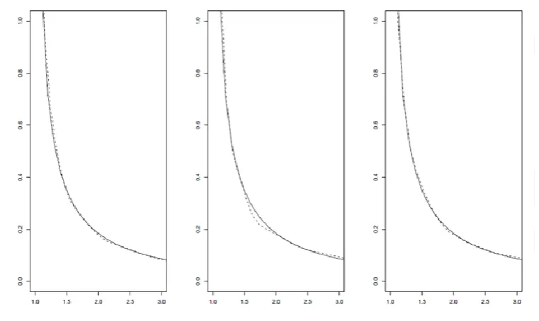
Figure. 1. True density, black line and its estimates
f
n,
dashed line, for Weibull distribution with , ,9 . 0 , 75 . 0 , 6 . 0
sequence
k
(
n
)
, we consider an arbitrary consistency result holding for the estimator with kernelK
(that satisfies Assumption A3) and bandwidth.
)/
(
=
k
n
n
h
n Then this result holds for the nearestneighbor estimator with kernel
K
and the bandwidth based onk
(
n
)
. The only prerequisite for this argument is that the conditions onh
n must also besatisfied by
h
n for any
>
0
.Theorem 1. Under Assumptions A1-A4 and A5(i),
(iii) , (iv), for
a
y
b
, we have.
.
0
=
]
)
(
)
(
[
lim
f
ny
f
y
a
s
n
(11)
Proof. See Appendix.
In what follows, we prove strong uniform consistency of the nearest neighbor density
estimator in the RLT model.
Theorem 2. Under Assumptions A1-A4 and A5 (i),(ii),
.
.
0
|=
)
(
)
(
|
sup
lim
f
ny
f
y
a
s
b y a n
(12)
Proof. See Appendix.
1.2. Asymptotic Normality
Let f* be a density function of F* and
).
(
)
(
)
(
1
=
)
(
~
*u
dF
y
R
u
y
K
y
R
y
f
nn n
n
To state and prove the asymptotic normality, we need the following assumption on density function of observed data.
A6:
(
k
(
n
))
1/2
f
*(
x
n)
f
*(
x
)
0,
in probability, when|
x
n
x
|=
O
(
k
(
n
)/
n
).
Theorem 3. Under Assumptions A1-A4, A5 (i)-(ii), and A6, for
a
y
b
, we have
(
)
(
)
(0,
(
)),
))
(
(
k
n
1/2f
ny
f
y
N
2y
D
(13) where
.
)
(
)
(
2
=
)
(
2 22
dy
y
K
y
f
y
Proof. See the Appendix.
Remark 1. We observe that asymptotic variance of
n
f
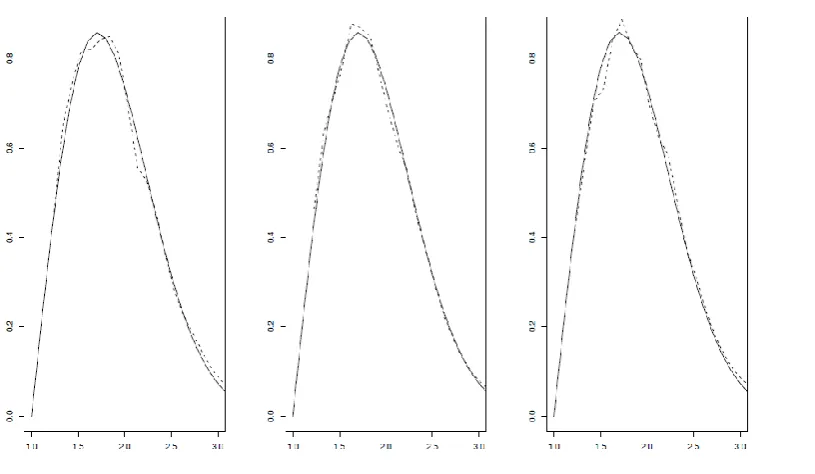
does not depend on truncation distribution.Figure. 2. True density, black line and its estimates
f
n,
dashed line, for Weibull distribution with,
9
.
0
,
75
.
0
,
6
.
0
Remark 2. A sufficient condition for Assumption
A6 to be true is that
f
* has an abounded derivative in a neighborhood ofa
y
b
,
in turn is satisfiedwhen
k
(
n
)
=
o
(
n
2/3).
This suboptimal choice for)
(
n
k
was used by Mielniczuk [13] in the randomcensorship model.
Remark 3. In complete data, the best rate for
)
(
n
k
is obtained aboutn
4/5 (in MSE sense, see e.g.,Mack and Rosenblatt, [12]).
Corollary 1. It is possible to construct confidence
interval for
f
using Theorem 3. For that purpose, aplug-in estimate
,
)
(
)
(
2
:=
)
(
2 22
dy
y
K
y
f
y
nn
for the asymptotic variance
2(
y
)
can be easily obtained using (10). This is a consistent estimator and yields a confidence interval of asymptotic level1
,
namely,
(14)
( ) ( )/ ( ) , ( ) ( )/ ( ) 1 /2
,1/2 2
/2 1 1/2 2
y k n z f y y k n z y
fn n n n
where
z
1/2 denotes the(1
/2)
quantile of the standard normal distribution.Application
1.Simulation
To show the performance of the proposed estimator, we present simulated models to compute the estimator fn(x) that is presented in
(10)
. We simulatedN
i
.
i
.
d
.
random variables(
Y
i,
T
i)
.
Here it is assumed that truncating variable is distributed as an exponential random variable with parameter
.
The exponential parameter is needed to obtain differentvalues of the theoretical proportion. The variable
Y
is distributed as a Weibull distribution with density
for and
and, a mixture distribution with the following density function
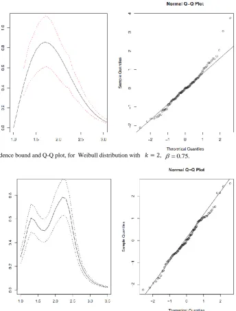
Figure. 3. True density, black line and its estimates
f
n,
dashed line, for mixtur distribution, 0.6,0.75,0.9, respectively.Figure. 4. Confidence bound and Q-Q plot, for Weibull distribution with , 0.75. Figure. 5. Confidence bound and Q-Q plot, for Weibull distribution with , 0.75.
y>1.
We then kept the data
(
Y
i,
T
i)
such thatY
i
T
i.
Using this scheme,m
10
independent samples of sizen
were generated. For each sample, plug-in estimates
n and for and were used respectively. The following figures represent the average ofm
density estimations and their the confidence bounds. The kernel function
1
|
|
(
),
81
70
=
)
(
x
x
3 3I
(||1)x
K
x(15)
where
I
A(
x
)
is indicator function for setA
, is used to construct a density estimator. It should be noted that the applied kernel(15)
satisfies the Assumption A3. In the case wheren
=
500,
we give the confidence bound and Q-Q plot.As one can see from Figures 1, 2 and 3, the quality of the estimator does not seem to be affected by
.
By employing
(13),
95%
asymptotic confidence band for the true Weibull distributions and mixture model are constructed and plotted in Figures 4, 5 and 6.According to the Q-Q- normal plots, we trivially notice that
(2)
(2))
(2)
(
)
(
(
1/2n
n
f
f
n
k
has asymptotically standard Normal distribution. Furthermore Kolmogorov-Smirnov test gives the p-values 0.59, 0.7892, 0.9306 respectively, for Weibull distributions with k=0. 5, 2 and mixture distribution, which suggests not to reject the Normality distribution.
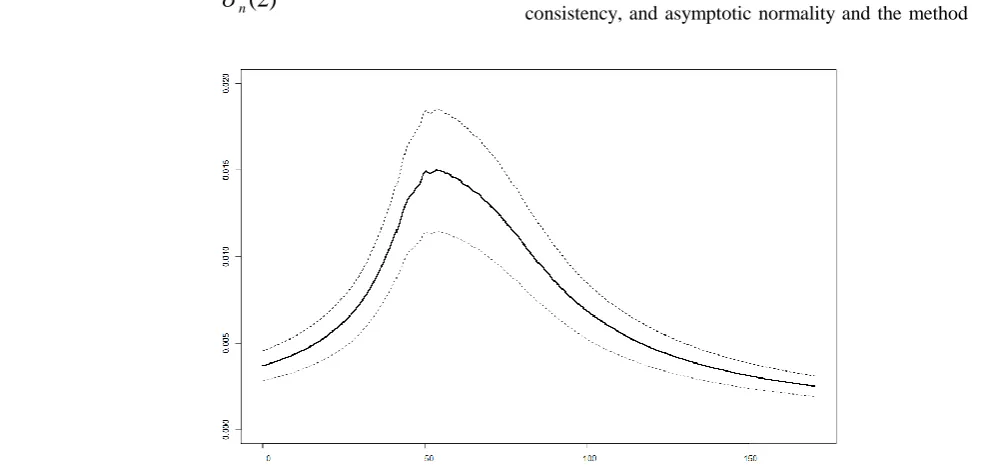
2.Real Data
In this subsection, a real data set of length-biased lifetimes with a size of 98 is used in order to estimate the density function . These are real data that are mentioned here from [9] and are recruited from brake pads in 1000 kilometer units. It should be mentioned that the length-biased data are special cases of left-truncation data when has a uniform distribution. We regenerated these data 10 times and the average of 10 density estimators is obtained. The estimator is graphed in Figure 7 in addition to the 95% confidence band for the true density. This confidence band is formulated in (14). It should be mentioned that these data appear to be distributed as Gamma distribution.
Conclusion
In this paper, a nearest neighbor kernel density estimator is proposed for the density function in the Left-truncation model. Uniform strong consistency and asymptotic normality of the proposed estimator is established. The performance of the estimator is illustrated through simulation studies. All simulations are drawn for different cases to demonstrate both consistency, and asymptotic normality and the method
is illustrated by real automobile brake pad data.
Appendix
In order to make the proofs easier, we need some auxiliary results and notation.
Lemma 1. Under Assumptions A1, A2, A4 and A5 (i) ,(iii), for
a
y
b
,
we have
(
)
(
)
.
.
)
(
2
)
(
s
a
y
G
y
f
y
nR
n
k
n
(16)Proof. Since distribution
F
* has a density which is continuous at pointy
,
by Theorem 1 ofMoore and Yackel [15] we obtain the result. Lemma 2. Under Assumptions A1-A2, A3(i), A4
and A5(i) , (iii), for
a
y
b
,
we have. . ) ( loglog log = ) ( ~ ) ( )
( as
n n k O n n n O y f y G y
fn n
Proof. Let
S
(
y
,
r
)
=
{
x
:|
x
y
|
r
}
, we have] ) ( ) ( [ ) ( ) ( 1 |= ) ( ~ ) ( ) ( | 1
= G y n
Y a y R Y y K y R y f y G y
f n i
n i n i n n n
|, ) ( ) ( | max ) ( ) ( ) ( sup )) ( ,( G y
Y na y nR n k y
K n i
y n R y S i Y n y (17)
where
a
n(
Y
i)
is the value of the jump of the Lynden-Bell estimator inY
i,
that is)
(
)
(
=
)
(
i n i
n in
Y
F
Y
F
Y
a
( ),) ( 1
= n i
i n Y F Y nC (18)
where
F
n= 1
F
n,
and ( )=(cf. Woodroofe, [25]).
Now, using Lemma 1 it is enough to show that
. . ) ( loglog log |= ) ( ) ( | max )) ( , ( s a n n k O n n n O y G Y nan i y n R y S i Y (19) By using (18), we have
| ) ( ) ( 1 ) ( ) ( 1 | max | ) ( ) ( | max )) ( , ( )) ( , (
SyRny n i Yi SyRny n i n i i n i i Y Y F Y C Y F Y C y G Y na | ) ( ) ( 1 ) ( ) ( 1 | sup )) ( , (
S yRn y C Fn C F . |=: ) ( 1 ) ( 1 |
sup 1 2 3
)) ( , ( I I I G y G y n R y S (20)
It is easy to see that
. ) ( ) ( max ) ( inf | ) ( ) ( | sup ) ( 2 1 i n i y n R y i Y b y a n Y C Y C y C C C I
Note that
inf
aybC
(
y
)
>
0.
By (4), (5) and theclassical Law of the Iterated Logarithm for empirical processes, (see for example [5]) we have
.
.
,
loglog
|=
)
(
)
(
|
sup
a
s
n
n
O
C
C
n
hence, by Corollary 1.3 of Stute [21]
.
.
,
loglog
log
=
1
a
s
n
n
n
O
I
(21)To deal with
I
2, by Corollary 2.2. of Zhou and Yip [28] and for large enoughn
, we have| ) ( ) ( | sup ) ( inf ) ( < < 1
2
F F
y C I n y n R y F a b y a . . , loglog
= as
n n O (22)
Since
I
3 is majorized by
( ( ))
, )) ( ( )) ( ( 2 y R y G y R y G y R y G n n n then it follows from
. . ), ( 2 ) ( )) ( ( )) ( ( s a y g y R y R y G y R y G n n n
and ., . (1), = ) ( ) ( s a O n k y nRn that . . , ) ( =
3 as
Now using (20)-(23), we obtain (19), and we get the result.
The following lemma can be easily obtained by the main result of Devroye and Wagner [6].
Lemma 3. Under Assumptions A1, A2, A4 and
A5 (i), (ii)
.
.
0
|
)
(
)
(
2
)
(
)
(
|
sup
f
y
G
y
a
s
y
nR
n
k
n b y a
(24)Proof of Theorem 1. Using Lemma 2, and the result of Nadaraya [17] we obtain the result.
Proof of Theorem 2. First, we show that the strong convergence in Lemma 2 can be replaced by uniform strong convergence on
[
a
,
b
].
To prove this, it is enough considering the last term of the majorant occurring in the proof of Lemma 2 and to show that
( )
( )
= ( ) ..sup as
n n k O y R y G y R y
G n n
b y a We have )) ( ( )) ( (
supG y Rn y G y Rn y
b y a
)
(
))
(
(
))
(
(
)
(
)
(
)
(
sup
=
y
R
y
R
y
G
y
R
y
G
n
k
y
nR
n
n
k
n n n n b y a
Since by Lemma 3,
sup
yR
n(
y
)
on[
a
,
b
]
tendsto 0 a.s. and
g
is uniformly continuous, we have. . 0 | ) ( 2 ) ( )) ( ( )) ( ( |
sup g y as
y R y R y G y R y G n n n b y a
Thus the proof of Theorem 1 is completed in view of Lemma 3, Theorem
A
of Silverman [20] and thefact that
f
.
G
is positive on[
a
,
b
].
Proof of Theorem 3. Observe that for
~
f
n(
y
)
, we have (25)
K ydyy G y f N y G y f y f n
k n ( )
) ( ) ( 0,2 ) ( ) ( ) ( ~ )) ( ( 2 2 1/2 D
(Moore and Yackel [15]).
(13)
follows from (25) and Lemma 2.References
1. Andersen P.K., Borgan O., Gill R.D., Keiding N. Statistical models based on counting processes. Springer, New York. (1993).
2. Biau G., Chazal F., Cohen-Steiner D., Devroye L. and Rodríguez, C., A weighted k-nearest neighbor density estimate for geometric inference, Elect. J. Statist. 204– 237 (2011).
3. Chen K., Chao M.T. and Lo S.W., On strong uniform consistency of the Lynden-Bell estimator for truncated data, Ann. Statist.23: 440–449 (1995).
4. Cs gŐ M. d Szy zk w cz B., L m m nearest-neighbor density estimation under long-range dependence, J. Stat. Reasarch.39: (1): 115–132 (2005). 5. Cs gŐ M. d Révé z P. S g App m Probability and Statistics. Academic Press, New York. (1981).
6. Devroye L.P. and Wagner T.J., The strong uniform consistency of nearest neighbor density estimates, Ann. Statist.5: 536–540 (1977).
7. He S. and Yang G.L. Estimating a lifetime distribution under different sampling plan. In: Gupta, S. S. and Berger, J. O. (eds.), Statistical Decision Theory and Related Topics, Springer, New York. 5: 73–85 (1994). 8. Keiding N. and Gill R.D., Random truncation models
and Markov processes, Ann. Statist.18: 582–602 (1990). 9. Lawless, J.F. Statistical Models and Methods for Lifetime Data. Ed ., John Wiley & Sons, New York, pp 69-70 (2003).
10. Loftsgaarden D.O. and Quesenberry C.P., A nonparametric estimate of a multivariate density function, Ann. Math. Statist.36: 1049–1051 (1965).
11. Lynden-Bell D., A method of allowing for known observational selection in small samples applied to 3CR quasars, Mon. Notices Roy. Ast. Soc.155: 95–118 (1971). 12. Mack Y.P. and Rosenblatt M., Multivariate
k
-nearest neighbor density estimates, J. Multi. Anal. 9: 1–15 (1979).13. Mielniczuk J., Some asymptotic properties of kernel estimators of a density function in case of censored data, Ann. Statist.14: 766–773 (1986).
14. Moore D.S. and Henrichon E.G., Uniform consistency of some estimates of a density function, Ann. Math. Statist. 40: 1499–1502 (1969).
15. Moore D.S. and Yackel J.W., Large sample properties of nearest neighbor density function estimators. In: Gupta, S. S. and Moore, D. S. (eds.), Statistical Decision Theory and Related Topics, Academic, New York. 269–279 (1976).
16. Moore D.S. and Yackel J.W., Consistency properties of nearest neighbor density estimates, Ann. Statist.5: 143– 154 (1977).
17. Nadaraya E.A., On nonparametric estimates of density functions and regression curves, Theor. Probab. Appl. 10:186–190 (1965).
the choice of optimal Tatra Mt. Math. Publ. 50: 39–45 (2011).
19. Ouadah S., Uniform-in-bandwidth nearest-neighbor density estimation, Stat. Prob. Lett. 83: (8):1835–1843 (2013).
20. Silverman B.W., Weak and strong uniform consistency of the kernel estimates of a density and its derivatives, Ann. Statist.6: 177–184 (1978).
21. Stute W., Almost sure representation of the product-limit estimator for truncated data, Ann. Statist. 21: 146–156 (1993).
22. Tsai W.Y., Jewell N.P. and Wang M.C., A note on the product-limit estimator under right censoring and left
truncation, Biometrika.74: 883–886 (1987).
23. Wagner T. J., Strong consistency of a nonparametric estimate of a density function, IEEE Trans. Systems, Man, and Cybernet.3: 289–290 (1973).
24. Wang M.C., Jewell N.P. and Tsai W.Y., Asymptotic properties of the limit-product estimate under random truncation, Ann. Statist.14: 1597–1805 (1986).
25. Woodroofe M., Estimating a distribution function with truncated data, Ann. Statist.13: 163–177 (1985). 26. Yang S.C., Consistency of nearest neighbor density
27. Yanyan L. and Yanli Z., The consistency and asymptotic normality of nearest neighbor density estimator under
-mixing condition, Acta Math. Scientia. 30: (3): 733–738 (2010).28.
Zhou Y. and Yip P.S.F., A strong representation of the