Numerical Solution of Nth-Order Fuzzy Differential Equations by Third Order Runge Kutta Method Based on Combination of Arithmatics, Harmonics and Geometrics Means

(1)

Numerical Solution of N

th

-Order Fuzzy Differential

Equations by Third Order Runge Kutta Method Based on

Combination of Arithmatics, Harmonics and Geometrics

Means

Yanti Rini1,*_{, Hajjah Alyauma}2

1_{Department of Informatics, STMIK Amik Riau, Pekanbaru, Indonesia} 2_{Department of Informatics, STIKOM Pelita, Pekanbaru, Indonesia}

Abstract

We discuss a numerical solution of Nth_{-order fuzzy differential equations with initial value by third order Runge} Kutta method based on combination of arithmatics, harmonics and geometrics means. Moreover, the convergence, stability and error analysis also discussed. The algorithm is illustrated by solving the Nth_{-order of fuzzy initial value problem. The} numerical simulation show that the new method worked and give an accurate solution.

Keywords

Fuzzy numbers, Nth_{-order fuzzy Initial value problem, Runge Kutta method, Lipschitz condition}

1. Introduction

Every physical problem is inherently biased by uncertainty. There is often a need to model, solve, and interpret the problems one encounters in the world of uncertainty. To overcome this uncertainty and vague, we may use the interval and fuzzy set theory. The topic of fuzzy differential equations (FDEs) forms a suitable setting for mathematical modelling of this physical problems. The concept of fuzzy derivative was first introduced by Chang and Zadeh (1972). Numerical solution for linear fuzzy differential equation was studied by many researcher ([1], [2], [3], [4], [5], [6], [7], [8], [9]). The solution of n-th order of fuzzy differential equation also derive by [10], [11], [12], [13] and [14]. The most frequently method to get the numerical solution is Runge Kutta method.

This paper studied a third order Runge Kutta method based on combination of arithmatics, harmonics and geometrics mean to solve n-th order of fuzzy initial value problem. In the Section 2, we begin with some preliminary results and concepts about fuzzy number and system of fuzzy initial value problem. In Section 3, we discuss the main idea to solve the problem. We also analyse the stability, convergence and the error, then we employ the

* Corresponding author:

[email protected] (Yanti Rini) Published online at http://journal.sapub.org/am

Copyright©2018The Author(s).PublishedbyScientific&AcademicPublishing This work is licensed under the Creative Commons Attribution International License (CC BY). http://creativecommons.org/licenses/by/4.0/

method on test example. Finally, in Section 4 we give the conclusion of this study.

2. Preliminaries

2.1. A Fuzzy Number

An interval

~

x

is denoted by

[ ]

x

,

x

on the set of real numbers R given by

[ ]

x

{

x

R

x

}

x

=

,

=

∈

:

≤

~

_.

In this paper, we have only considered closed intervals, although there exist various types of intervals such as open and half-open intervals. A fuzzy number

U

~

is convex, normalized fuzzy set

U

~

of the real line

R

such that

( )

[ ]

{

µ

_U~

x

:

R

→

0 1,

,

∀

x

∈

R

}

,

where,

µ

_U~ is called the membership function of the fuzzy set, and it is piecewise continuous. A triangular fuzzy number

v

is defined by three numbers

a

₁

<

a

₂

<

a

₃, where the graph of

v

( )

x

, the member of function of the fuzzy number

v

, is a triangle with the base on the interval

[

a

₁

,

a

₃

]

and the vertex at

x

=

a

2 . We specify

v

as

(2)

i.

v

>

0

if

a

1

>

0

; ii.

v

≥

0

if

a

1

≥

0

; iii.

v

<

0

if

a

₃

<

0

and iv.

v

≤

0

if

a

₃

≤

0

.

Let

E

be a set of all the upper semicontinuous normal convex fuzzy numbers with bounded r-level sets. It means that if

v

∈

E

, then the

r

-level set

[ ]

v

r

=

{

s

|

v

( )

s

≥

r

}

,

0 <

r

≤

1

, is a closed bounded interval which is denoted by

[ ]

v

r

=

[

v

1

( ) ( )

r

,

v

2

r

]

.

Let

I

be a real interval. The mapping

x

:

I

→

E

is called fuzzy process and its

r

-level set is denoted by

( )

[ ]

x

t

r

=

[

x

₁

( ) ( )

t

;

r

,

x

₂

t

;

r

]

,

t

∈

I

,

r

∈

(

0 ,

1 ]

. The derivative

x

'

( )

t

of the fuzzy process

x

is defined by

( )

[ ]

x

'

t

r

=

[

x

1

'

( ) ( )

t

;

r

,

x

2

'

t

;

r

]

,

t

∈

I

,

r

∈

(

0 ,

1 ]

, provided that this equation determines the fuzzy number.

Let

κ

be the set of all nonempty compact subset of

R

and

κ

_c be the subset of

κ

consisting of nonempty convex compact sets. Recall that

(

,

)

min

A

x A

x a

α

ρ

∈

=

−

is a distance of the point

x

∈

R

from

A

∈

κ

and that the Hausdorff separation

ρ

(

A

,

B

)

of

A

,

B

∈

κ

is defined as

(

,

)

max

(

,

)

A

A B

a B

α

ρ

∈

=

.

2.2. A nth_{Fuzzy Initial Value Problem} Consider the fuzzy initial value problem

( )

(

( )

)

( )

_{( )}









=

−

,

0 ,

,

0 ,

,

,'

,

1 1

1

n n

a

x

a

x

t

x



ϕ

(1)

where

ϕ

is continuous mapping from

R

+

×

R

n into

R

and

a

_i

(

0 ≤

i

≤

n

)

are fuzzy numbers in

E

. The

n

th

-order fuzzy differential equation by changing variables

( ) ( ) ( )

_,

_'

( )

_,

( )

( 1)

_{( )}

_,

2

1

t

x

t

y

t

x

t

y

t

x

t

y

n

=

−

=



converts to the following fuzzy system

( )

(

)

( )

(

)

( )

[ ]

_{( )}

[ ]











=

,

0 ,

,

0 ,

,

'

,

'

0 1

0 1 1

1 1 1 1

n n n

n n

n

a

y

a

y

t

f

t

y

t

f

t

y







(2)

where

f

_i

(

1 ≤

i

≤

n

)

are continuous mapping from

n

R

₊

×

into

R

and

y

[ ]_i0 are fuzzy numbers in

E

with

α

-level intervals

[ ]

y

i[ ]0 _α

=

[

y

_i[ ]0

( )

α

,

y

_i[ ]0

( )

α

]

for

,

1 n

i

=



and

0 <

α

≤

1 .

Now, we have to show that the solution of (2) is

(

)

t

n

y

=

1

,



,

on a interval

I

, if

( )

{

(

)

[

( ) ( )

]

}

( )

(

,

)

,

;

,

min

,

₁

'

α

t

y

t

f

t

y

t

y

u

t

f

t

y

i

j j

j n i

i

=

∈

=



( )

{

(

)

[

( ) ( )

]

}

( )

(

,

)

,

;

,

max

,

1

'

α

t

y

t

f

t

y

t

y

u

t

f

t

y

i

j j

j n i

i

=

∈

=



and

( )

0 ,

_α

[ ]0

( )

_α

,

( )

0 ,

_α

[ ]0

( )

_α

.

i i

i

y

=

For fixed value

α

, we have a system of initial value problem in

R

2n and we have intervals

( ) ( )

[

y

_j

t

,

α

,

y

_j

t

,

α

]

with a fuzzy number

y

_i

( )

t

∈

E

. Let [ ]

_{( )}

(

[ ]

_{( )}

[ ]

_{( )}

)

t

n

i

y

0

α

₌

0

α

_,

_

_,

0

α

and

[ ]

_{( )}

(

[ ]

_{( )}

[ ]

_{( )}

)

t n

i

y

0

α

=

0

α

,



,

0

α

,

with respect to the indicators system (2) can be written as with assumption

( )

(

( )

)

( )

[ ]







∈

=

.

0 ,

,

'

0

_E

n

y

t

y

t

F

t

y

(3)

With assumption

y

( )

t

,

α

=

[

y

( ) ( )

t

,

α

,

y

t

,

α

]

and

( )

,

α

[

'

( ) ( )

,

α

,

'

,

α

]

'

t

y

t

y

t

y

=

where

( )

_t

,

(

_y

( )

_t

,

_y

( )

_t

,

)

t

,

y

α

=

α

_

α

( )

t

,

(

y

( )

t

,

y

( )

t

,

)

t

,

y

α

=

α



α

( )

,

(

'

( )

,

'

( )

,

)

,

'

_t

_y

_t

_y

_t

t

y

α

=

α



α

( )

,

(

'

( )

,

'

( )

,

)

,

'

t

y

t

y

t

y

α

=

α

_

α

and

F

(

t

,

y

( )

t

,

α

)

=

[

F

'

(

t

,

y

( )

t

,

α

)

,

F

'

(

t

,

y

( )

t

,

α

)

]

, where

( )

(

,

)

(

₁

(

,

( )

,

)

,

(

,

( )

,

)

t

,

n

t

y

t

f

t

y

t

f

t

y

t

F

α

=

α

_

α

( )

(

,

)

(

1

(

,

( )

,

)

,

(

,

( )

,

)

.

t n

t

y

t

f

t

y

t

f

t

y

t

F

α

=

α

_

α

(3)

( )

(

( )

)

( )

(

( )

)

( )

[ ]

_{( ) ( )}

[ ]

_{( )}











=

.

,

0 ,

,

0 ,

,

'

,

'

0

_α

α

y

t

y

t

F

t

y

t

y

t

F

t

y

(4) Or

( )

(

( )

)

( )

[ ]

_{( )}







=

.

,

0 ,

,

'

0

_α

α

y

t

y

t

F

t

y

(5)

Theorem 2.1. If

f

_i

(

t

,

u

₁

,



,

u

_n

)

for

i

=

1 ,



,

n

are continuous function of

t

and satisfies the Lipschitz condition in

u

=

(

u

1

,



,

u

n

)

t in the region

( )

[ ]

{

t

u

t

u

i

n

}

D

=

,

∈

0 1,

,

−∞

<

i

<

∞

for

=

,1



,

with

constant

L

_i then the initial value problem (2) has unique solution in each case.

Proof. See [15]

By Theorem 3.1 the initial value problem (2) has a unique solution

y

=

(

y

1

,



,

y

n

)

t.

2.3. Runge Kutta Method

The basis of all Runge Kutta method of order m is to express the difference between the value of

t

n+₁ and

t

n as

1

0

m

n n i i

i

y

+

y

w k

=

−

=

∑

where

w

_i

'

s

are constants and

1

,

i

.

i n i n ij j

j

k hf t

a h y

−

c k

=





=



_

+



_



∑



The Runge Kutta method of order 3 based on combination of arithmetic, harmonic and geometric means is [16]

(

)

(

))

,

32

2

7

90

3 2 2 1 3 2 3 2 2 1 2 1 3 2 1 1

k

h

y

n n

+













+

−

+

=

+ (6) with

(

,

)

,

1

f

t

n

y

n

k

=

, 3 2 , 3 2 1 2       ₊ ₊

= f t h y hk

k n n

.

9

10

9

4 ,

3

2

2 1 3













₊

₋

₊

=

f

t

h

y

h

k

h

k

n n

3. The Third Order of Runge Kutta

Method Based on Combination of

Arithmatics, Harmonics and

Geometrics Mean

Define

(

) (

)

(

)

(

) (

)

(

)

3 1 ,1 1 3 1 ,2 1

;

,

;

,

;

,

;

,

n n i i n n

i

n n i i n n

i

y t

w k t y t

y t

w k

t y t

α

+ + = =

−

=

−

=

∑

( )

(

)

[

]

[

(

( )

)

(

( )

)

]

.

3 ,

2 ,1

,

;

,

;

,

_,₁ _,₂

=

i

t

y

t

k

t

y

t

k

t

y

t

k

i

α

α i

α

i

α

(

)

(

)

(

( )

(

)

(

)

,1 1 1 ,1 1

;

,

;

i n n n i n

i

ij j n n

j

k t y t

h f t

a h y t

b k

t y t

α

− =

= ⋅

+

∑

(

)

(

)

(

( )

(

)

(

)

,2 2 1 ,2 1

;

,

;

.

i n n n i n

i

ij j n n

j

k

t y t

h f t

a h y t

b k

t y t

α

− =

= ⋅

+

∑

With

( )

(

)

{

(

)

( ) ( )

[

]

}

(

i

n

)

(4)

( )

(

)

( ( ) )

[

( ( ) )

,

;

,

]

}

.

,

;

,

3 max

;

,

2 , 2 1 , 2 1 2 , 3

h

t

y

t

z

h

t

y

t

z

s

h

t

f

h

t

y

t

k

i n

α

∈

















 +

⋅

=

_

By the third order Runge Kutta based on combination of means, we obtain

( )

(

)

( )

(

,

( )

;

)

, 3 2 ; , ;

, 1 1,1

1 ,

1 t y t

α

h y t

α

k t yt

α

z = +

( )

(

)

( )

(

,

( )

;

)

, 3 2 ; , ;

, 2 1,2

2 ,

1 t yt α h y t α k t ytα

z = +

( )

(

)

( )

(

( )

)

( )

(

, ; ,

)

, 9 10 , ; , 9 4 ; , ; , 1 , 2 1 , 1 1 1 , 2 h t y t k h t y t k t y h t y t z α α α α + − =

( )

(

)

( )

(

( )

)

( )

(

, ; ,

)

. 9 10 , ; , 9 4 ; , ; , 2 , 2 2 , 1 2 2 , 2 h t y t k h t y t k t y h t y t z

α

+ − =

From Eq. (6), define

( )

(

) (

(

( )

)

(

( )

)

( )

(

)

( )

(

)

(

( )

)

( )

(

)

(

( )

)

( )

(

)

(

( )

)

( )

(

)

(

( )

)

( )

(

)

(

( )

)

(

( )

(

t yt h

)

k

(

t y

( )

t h

)

))

k h t y t k h t y t k h t y t k h t y t k h t y t k h t y t k h t y t k h t y t k h t y t k h t y t k h t y t k h t y t k h t y t k h t y t F , ; , , ; , , ; , , ; , 32 , ; , , ; , , ; , , ; , 2 , ; , , ; , , ; , , ; , 2 , ; , , ; , 2 , ; , 7 , ; , 1 , 3 1 , 2 1 , 2 1 , 1 1 , 3 1 , 2 1 , 3 1 , 2 1 , 2 1 , 1 1 , 2 1 , 1 1 , 3 1 , 2 1 , 1

α

+ + + +     + +     + − + + = and

( )

(

) (

(

( )

)

(

( )

)

( )

(

)

( )

(

)

(

( )

)

( )

(

)

(

( )

)

( )

(

)

(

( )

)

( )

(

)

(

( )

)

( )

(

)

(

( )

)

(

( )

(

, ; ,

)

(

,

( )

; ,

)

))

. , ; , , ; , 32 , ; , , ; , , ; , , ; , 2 , ; , , ; , , ; , , ; , 2 , ; , , ; , 2 , ; , 7 , ; , 2 , 3 2 , 2 2 , 2 2 , 1 2 , 3 2 , 2 2 , 3 2 , 2 2 , 2 2 , 1 2 , 2 2 , 1 2 , 3 2 , 2 2 , 1 h t y t k h t y t k h t y t k h t y t k h t y t k h t y t k h t y t k h t y t k h t y t k h t y t k h t y t k h t y t k h t y t k h t y t k h t y t k h t y t G α α α α α α α α α α α α α α α α + + + +     + +     + − + + =

The discrete equally spaced grid points

{

t

0

=

0 ,

t

1

,



,

t

N

=

T

}

is a partition for interval

[ ]

0 ,

T

.

If the exact and the approximate solution in the

i

-th

α

cut

at

t

_m

,

0 ≤

m

≤

N

are denoted by

[

y

[ ]_im

( )

α

,

y

_i[ ]m

( )

α

]

and

[

Y

[ ]_im

( )

α

,

Y

i[ ]m

( )

α

]

respectively, then the numerical

solution by third order Runge Kutta method based on combination of arithmetic, harmonics and geometrics means is [ ]

_{( )}

[ ]

_{( )}

(

_{( )}

)

[ ]

_{( )}

[ ]

_{( )}

_, , , , 90 0 0 1

α

i i m m i m i m i y Y h Y t F h Y Y = + = + [ ]

_{( )}

[ ]

_{( )}

₍

_{( )}

₎

[ ]

_{( )}

[ ]

_{( )}

, , , , 90 0 0 1

α

i i m m i m i m i y Y h Y t F h Y Y = + = +

with

[ ]

Y

_i

( )

t

_α

=

[

Y

_i

( ) ( )

t

,

α

,

Y

i

t

,

α

]

,

[ ]_m

_{( )}

_α

[

[ ]_m

_{( )}

_α

[ ]m

_{( )}

_α

]

Y

=

,

[ ]

_{( )}

(

[ ]

_{( )}

[ ]

_{( )}

)

[ ]

_{( )}

(

[ ]

_{( )}

[ ]

_{( )}

)

.

,

1 1 t m n m m t m n m m

Y

and

Y

α



=

Let [ ]

_{( )}

(

)

(

[ ]

_{( )}

)

[ ]

_{( )}

(

,

))

,

90

1 ,

,

*

1 t m n m m

h

Y

t

F

h

Y

t

F

h

Y

t

F

α

=

_

[ ]

_{( )}

(

)

(

[ ]

_{( )}

)

[ ]

_{( )}

(

, ,

))

. , , , , 90 1 , , * 1 t m n m m h Y t G h Y t G h Y t G

α

= _

The approximate solution for

α

-cut of Eq.(2) is [ ]

_{( )}

[ ]

_{( )}

(

[ ]

_{( )}

)

[ ]

_{( )}

_α

[ ]

_{( )}

_α

α

0 0

1

_,

y

Y

h

Y

t

hH

Y

m m m m

=

+

=

+ (7) where [ ]

_{( )}

(

)

[

(

[ ]

_{( )}

)

[ ]

_{( )}

(

,

)

]

,

*

,

*

,

h

Y

t

G

h

Y

t

F

h

Y

t

H

m m m m m m

α

=

and [ ]

_{( )}

(

)

(

[ ]

_{( )}

)

(

[ ]

_{( )}

)

[ ]

_{( )}

(

)

[ ]

_{( )}

(

)

(

[ ]

_{( )}

)

[ ]

_{( )}

(

)

(

[ ]

_{( )}

)

1 2 3 1 2 1 2 * , ,

1 7 , , 2 , ,

90

, ,

2 , , , ,

, , , , m m m m m m m m m m m m m m m m

F t Y h

k t Y h k t Y h

k t Y h

k t Y h k t Y h

(5)

[ ]

_{( )}

(

)

(

[ ]

_{( )}

)

[ ]

_{( )}

(

)

(

[ ]

_{( )}

)

[ ]

_{( )}

(

)

(

[ ]

_{( )}

)

(

[ ]

_{( )}

(

)

(

[ ]

_{( )}

)

2 3

1 2

2 3

2 , , , ,

, , , ,

32 , , , ,

, , , ,

m m

k t Y h k t Y h

k t Y h k t Y h

α

+

+ +







[ ]

_{( )}

(

)

(

[ ]

_{( )}

)

(

[ ]

_{( )}

)

[ ]

_{( )}

(

))

[ ]

_{( )}

(

)

(

[ ]

_{( )}

)

[ ]

_{( )}

(

)

(

[ ]

_{( )}

)

[ ]

_{( )}

(

)

(

[ ]

_{( )}

)

[ ]

_{( )}

(

)

(

[ ]

_{( )}

)

[ ]

_{( )}

(

)

(

[ ]

_{( )}

)

[ ]

_{( )}

(

)

(

[ ]

_{( )}

)

1 2

3

1 2

2 3

1 2

2 3

* , ,

1 7 , , 2 , ,

90

, ,

2 , , , ,

, , , ,

2 , , , ,

, , , ,

32 , , , ,

, , , ,

m m

G t Y h

k t Y h k t Y h

k t Y h

k t Y h k t Y h

α

= +

+

 

−_ ₊



 

+ _

+ 

 

+ _ +



 

+ + _



with

[ ]

_{( )}

(

)

(

[ ]

_{( )}

)

[ ]

_{( )}

(

,

))

,

1

t m

nj m j m

j

h

Y

t

k

h

Y

t

k

h

Y

t

k

α

=

_

[ ]

_{( )}

(

)

(

[ ]

_{( )}

)

[ ]

_{( )}

(

,

)

.

,

1

t m

nj m j m

j

h

Y

t

k

h

Y

t

k

h

Y

t

k

α

=

_

3.1. Stability, Convergence and Error Analysis

To analyse the stability, convergence and the error of the method, consider the next definition and theorem.

Definition 3.1. [15] A one-step method for approximating the solution of differential equation

( )

(

( )

)

( )

[ ]







∈

=

,

0 ,

,

'

0

_R

n

y

t

y

t

F

t

y

with

F

is a

_n

th

−

_{ordered as}

(

)

t n

f

=

1

,



,

and

(

i n

)

R

R R

f n

i: +× → 1≤ ≤ is a method that can be

written in the form

[ ]1

_Y

[ ]

_h

(

_t

_,

_Y

[ ]

_,

_h

)

_,

Y

n

n n

n+

₌

₊

_ϕ

(8)

where the increment function

ϕ

is determined by

F

.

Theorem 3.2. If

ϕ

(

t

,

y

,

h

)

satisfies a Lipschitz condition in

y

then the method given by (8) is stable.

Theorem 3.3. In relation (2), if

F

( )

t

,

y

satisfies a Lipschitz condition in y then the method given by (7) is stable.

Theorem 3.4. If

[ ]

_{( )}

[ ]

_{( )}

(

[ ]

_{( )}

)

[ ]

_{( )}

_α

[ ]

_{( )}

_α

α

ϕ

α

0 0

1 _, _, _,

y Y

h Y

t h Y

Y m

m m

m

=

+ =

+

where

[ ]

_{( )}

(

)

[

(

[ ]

_{( )}

)

[ ]

_{( )}

(

t

Y

h

)

]

h

Y

t

h

Y

t

m m

m m m

m

,

2 1

α

ϕ

α

ϕ

α

ϕ

=

Is a numerical method for approximation of differential equation (2),

ϕ

₁ and

ϕ

₂ are continuous in

t

,

y

,

h

for

,

0 ≤

t

≤

T

0 ≤

h

≤

h

₀ and all

y

, and if they satisfy a Lipschitz condition in the region

D

=

{

(

t

,

u

,

v

,

h

)

T

t

≤

0

,

−

∞

≤

u

_i

≤

v

_i,

−

∞

≤

v

_i

≤

∞

,

0 ≤

h

≤

h

₀,

}

n

i

=

0 ,



,

, the necessary and sufficient conditions for convergence is

( )

(

,

α

,

)

(

,

( )

,

α

)

.

ϕ

t

y

t

h

=

F

t

y

t

Proof. See [15].

Then the method proposed by (6) is convergent to the solution of the system (2).

3.2. Numerical Examples

The next example show the performance the new method.

Figure 1

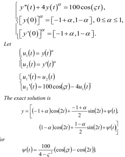
Example [15]. Consider the vibrating mass (

m

=

1

slug) in Fig.1. The spring constant is k =4lb _ft, there is no

damping force and the forcing function is 100cos

( )

ς

t for

0 >

(6)

( )

'' 4 100cos ,

0 1 ,1 , 0 1,

' 0 1 ,1 .

y t y t t

y y

α α

α

ς

α

 

   

   



_ _ _ _



+ =

= − + − ≤ ≤

= − + −

Let

( ) ( )

( )









=

α α

t

y

t

u

t

y

t

u

'

2 1

( )

100cos

( )

4

( )

. '

'

1 2

2 1

  

− =

=

t u t t

u

t u t u

ς

The exact solution is

(

) ( )

( ) ( )

(

−

) ( )

+ −

( ) ( )

+ _ 

₋ ₊ ₊− + ₊ =

t t t

y

ψ α

α

ψ α

α

2 sin 2 1 2 cos 1

, 2

sin 2 1 2 cos 1

for

( )

(

cos

( )

cos

( )

2

)

. 4

100

2 t t

t −

−

= ς

ς ψ

By using the new method, the numerical solution is in Table 1 and Table 2.

Table 1. The Solution of Example 1 for Y[ ]_im

( )

α

r Exact Numeric Error

0 -0.58756 -0.58734 0.00022

0.1 -0.48207 -0.47942 0.00265 0.2 -0.37658 -0.37146 0.00512 0.3 -0.27108 -0.26347 0.00761

0.4 -0.16559 -0.16459 0.001

0.5 -0.06011 -0.05821 0.0019

0.6 0.04538 0.04691 0.00153

0.7 0.15087 0.1581 0.00723

0.8 0.25636 0.26529 0.00893

0.9 0.36185 0.3722 0.01035

1 0.46734 0.479614 0.012274

Table 2. The Solution of Example 1 for Y[ ]im

( )

α

r Exact Numeric Error

0 1.57171 1.57143 0.00028

0.1 1.46622 1.46345 0.00277

0.2 1.36072 1.3555 0.00522

0.3 1.25523 1.24722 0.00801

0.4 1.14974 1.14514 0.0046

0.5 1.04425 1.03875 0.0055

0.6 0.93876 0.93363 0.00513

0.7 0.83372 0.82289 0.01083

0.8 0.72778 0.71525 0.01253

0.9 0.62229 0.60834 0.01395

1 0.51681 0.500936 0.015874

4. Conclusions

In this paper we presented a numerical approach to solve system of fuzzy differential equations with initial value. The scheme is based on the third order Runge Kutta method for solving n-th order of fuzzy initial value probrems. The stability, convergence and error analysis have been studied. Numerical simulation performs that the new method is an accurate method for n-th order of fuzzy initial value problems.

ACKNOWLEDGEMENTS

This works has fully supported by the Ministry of Research Technology and Higher Education of Indonesia.

REFERENCES

[1] Bede, B and Stefanini, L. 2011. Solution of Fuzzy Differential Equations with Generalized Differentiability using LU-Parametric Representation. EUSFLAT-LFA 2011. Juli 2011. Aix-les-Bains, France. 785-790.

[2] Buckley, J.J and Feuring, T. 2000. Fuzzy Differential Equations. Fuzzy Sets and Systems. 110. 43-54.

[3] Dhayabaran, D.P. 2015. A Method for Solving Fuzzy Differential Equations Using Runge-Kutta Method with Harmonic Mean of Three Quantities. International Journal of Engineering Science and Innovative Technology. 4(3). 90-96. [4] Ghanaie, Z.A and Moghdam, M.M. 2011. Solving Fuzzy

differential Equations by Runge-Kutta Method. The Journal of Mathematics and Computer Science. 2(2). 208-221. [5] Jayakumar, T, Maheskumar, D and Kanagarajan K. 2012.

Numerical Solution of Fuzzy Differential Equations by Runge Kutta Method of Order Five. Applied Mathematical Science. 6(60). 2989-3002.

[6] Jayakumar. T, Muthukumar. T and Kanagarajan. K. 2015. Numerical Solution of Fuzzy Differential Equations by Runge-Kutta Verner Method. Communcations in Numerical Analysis. 2015(1). 1-15.

[7] Rubanraj, S and Rajkumar, P. 2015. Numerical Solution of Fuzzy Differential Equation by Sixth Order Runge-Kutta Method. International Journal of Fuzzy Mathematical Archive. 7(1). 35-42.

[8] Yanti. R and Hajjah. A. 2017. Applied of Third Order Runge Kutta Method Based on Combination of Means to Solve Fuzzy Differential Equations. Proceeding of International Conference on Mathematics and Mathematics Educations (ICM2E) 2017. 2017(1). 291-299.

[9] Nieto. J, Khastan and Ivaz, K. 2009. Numerical Solution of Fuzzy Differential Equations under Generalized Differentiability. Nonlinear Analysis: Hybrid Systems. 3(40). 700-707.

(7)

by Runge Kutta Method. Mathematical and Computational Applications. 16(4). 935-946.

[11] Georgiou. D, Nieto, J and Rodriguez-Lopez, R. 2005. Initial Value Problems for Higher-Order Fuzzy Differential Equations. Nonlinear Analysis, Theory, Method and Applications. 63(4). 587-600.

[12] Jayakumar. T, Kanagarajan. K and Indrakumar, S. 2012. Numerical Solution of Nth-Order Fuzzy Differential Equation by Runge-Kutta Method of Order Five. Int. Journal of Math. Analysis. 6(58). 2885-2896.

[13] Siah Mansouri, S and Ahmady, N. 2012. A Numerical Method for Solving Nth-Order Fuzzy Differential Equation by using Characterization Theorem. Communication in Numerical Analysis. 12. 1-12.

[14] Jameel. A, Anakira, N.R, Alomari, K.A, Hashim, I and Shakhatreh, M.A. 2016. Numerical Solution of n’th Order Fuzzy Initial Value Problems by Six Stages. Journal of Nonlinear Science and Applications. 2016. 627-640.

[15] Abbasbandy, S. 2002. Numerical Solutions of Fuzzy Differential Equations by Taylor Method. Computational Method in Applied Mathematics. 2(2002). 113-124.