Volume 16, Number 4, pp. 423–435. http://www.scpe.org
ISSN 1895-1767 c
⃝2015 SCPE
SCALING BEYOND ONE RACK AND SIZING OF HADOOP PLATFORM
WIES LAWA LITKE∗AND MARCIN BUDKA†
Abstract. This paper focuses on two aspects of configuration choices of the Hadoop platform. Firstly we are looking to establish performance implications of expanding an existing Hadoop cluster beyond a single rack. In the second part of the testing we are focusing on performance differences when deploying clusters of different sizes. The study also examines constraints of the disk latency found on the test cluster during our experiments and discusses their impact on the overall performance. All testing approaches described in this work offer an insight into understanding of Hadoop environment for the companies looking to either expand their existing Big Data analytics platform or implement it for the first time.
Key words: Hadoop, Big Data analytics, scalability, benchmarking, teragen, terasort, teravalidate, inodes, platform bottle-necks, disk latency
AMS subject classifications. 11Y35, 20B40, 68, 68U, 93B40
1. Introduction. Hadoop is a distributed computational environment designed to facilitate storage and
analysis of large heterogeneous datasets (Big Data), which typically grow at high velocity [14]. It is a very sought after technology platform that many companies have either already deployed, are currently deploying or are looking to investing into. According to [15] the market penetration of Hadoop reached 32% among all enterprises at the end of 2014 and is predicted to grow to as much as 66% within the next two years.
One of the key components of the platform is the Hadoop Distributed File System (HDFS). Its roots stem from a simple problem: the transfer speeds of hard drives have not kept up with growing storage capacity. In 1990 a typical drive could store 1,370MB of data which could be accessed at 4.4 MB/s [14], so the contents of that drive could be read in just over five minutes. Two decades later, 1TB drives are the norm with access speeds of around 100MB/s taking almost 3 hours to read, which is an unacceptable bottleneck in the datacentre world, where the size of a typical dataset is measured in petabytes. Hadoop overcomes this limitation by simultaneously reading from multiple drives. 100 drives sharing an equal share of 1TB of data could be read in less than two minutes. This comes with a trade-off: higher risk of drive failure. Again this shortcoming is mitigated through storing multiple copies of files (replication). Analytics in this setting is facilitated by the MapReduce programming model which enables processing of large datasets via efficient parallelisation techniques [3], handling both structured and unstructured data that is complex, large and rapidly growing.
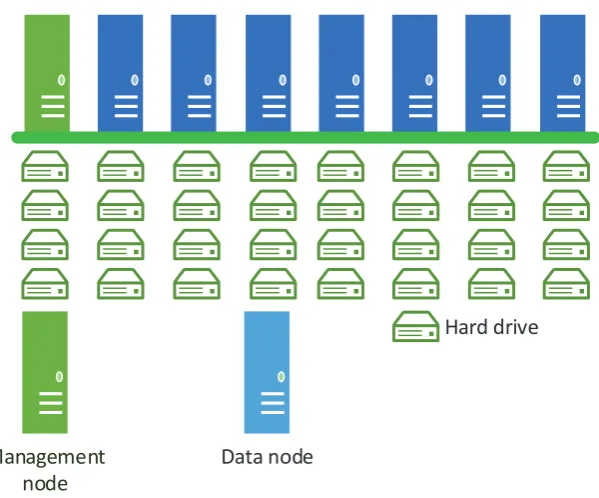
A typical architecture of a Hadoop cluster consists of a number of racks populated with commodity servers, referred to as nodes (cf. Fig. 1.1). Majority of those servers will be slave nodes (or data nodes) with a single master node (or management server), responsible for overseeing the key functionality of services such as HDFS or MapReduce [5]. The data nodes are normally populated with a moderate capacity of memory and storage (for details please refer to Sect. 2). Connectivity is provided via a high-throughput switch and boned network links.
Planning deployment of a Hadoop cluster involves consideration of hardware type, software choices, size (i.e. number of nodes) and anticipated load of the platform. If a business is looking to invest into Big Data analytics they face the problem of how considerable the investment should be, to deliver required storage and computational capacity to handle their workload. Future expansion also needs to be considered.
In this study we look into the scalability issues of the Hadoop platform and its impact on performance defined as time required to complete any given task. Two test scenarios have been devised:
1. Implications of scaling out a single-rack solution to a second rack. This scenario is applicable to businesses that already have an in-house Hadoop installation, however they need to expand. In this study we investigate expected performance improvements.
2. Performance of processing a workload as a function of the number of nodes at varying loads. This part of the study aims to aid the organisations with decision of size of the cluster that they want/need to
∗Intel Corporation, Pipers Way, Swindon Wiltshire SN3 1RJ, United Kingdom,[email protected]
†Faculty of Science and Technology, Bournemouth University, Fern Barrow, Talbot Campus, Poole, Dorset, BH12 5BB, United Kingdom,[email protected]
Management
node
Data node
Hard drive
Fig. 1.1: Cluster schematic diagram
implement.
The remainder of this paper is structured as follows. Sect. 2 briefly reviews related work. In Sect. 3 we outline the configuration of a cluster that was used to perform the experiments. The subsequent section describes in detail the chosen benchmark suite (TeraSort). The benchmark results and the performance of the cluster are reported in Sect. 5, while Sect. 6 contains analysis and discussion of the results. Finally, conclusions and outline of plans for future work can be found in Sect. 7.
2. Related work. When planning implementation of Hadoop cluster(s) the deployment model is one of
the most important decisions to make. Keeping Return of Investment (ROI) in mind the decision makers must choose whether to deploy on-premise hardware (bare metal), fully deploy in the Cloud or opt for something in between. Each of those options carries its own challenges and concerns. Five main deployment models are distinguished in [13]:
• On-premise full custom (bare metal) with Hadoop installed directly on companys hardware and the
business holding full control of data and cluster management.
• Hadoop appliance, which allows the business to jumpstart the data analysis process on a preconfigured
cluster owned by a third party operator.
• Hadoop hosting, where the service provider takes care of both cluster configuration and operation on
behalf of the client.
• Hadoop on the Cloud, which allows the business to create Hadoop environment on virtual machines
while maintaining full control as in bare metal.
• Hadoop-as-a-Service, in which the business is charged on pay-per-use basis.
2.1. Scaling beyond 1 rack. In [10] the author describes scalability as one of the most important
capabilities ideal for inevitable expansions of the platform.
Many analytic workloads require large memory resources to enable efficient search, read and write job execution. Unsurprisingly, I/O intensive in-memory operations outperform the ones that require hard drive access. However due to hardware constraints any commodity server would be limited in the available memory for analytic jobs processing. This is where the expansion of the cluster comes in. By adding additional racks an organisation can add extra pools of memory. However, that entails spreading the workload over multiple parallel servers, which can increase accompanying job coordination overheads.
When all those conditions are met and an organisation has installed new nodes as part of the cluster it is likely that the expanded cluster has become unbalanced [4]. Although new hardware is added to the platform, linked to the management server, and seen and recognised by the existing nodes, the data will stay where it is unless instructed otherwise. Job Tracker is a service that controls and assigns MapReduce jobs on the cluster. In order to avoid data shuffling between racks it will always assign jobs to run locally where the files are stored, if possible. This means that the MapReduce tasks are not going to be assigned to the new nodes unless the old nodes are at their maximum capacity. This results in underutilisation of the new resources.
Currently there are two tends for expanding the resources of the Hadoop cluster: scale out and scale up. The scale up option is based on adding additional storage devices to the existing rack and although it is the economical choice the cluster will rely on the same amount of management capabilities as before which may cause bandwidth issue. The scale out alternative adds both storage and performance to the existing environment which is what this paper focuses on. In [12] Sevilla presents a point where scaling up of the cluster affects its parallelism due to bottlenecks. In various tests he illustrates how scale up clusters work in sequential job phases and are outperformed by scale out clusters on which the jobs are parallelised. His point is being argued by Appuswamy [2] where he illustrates how to improve the performance of scale up by series of optimisations.
2.2. Scalability of nodes processing the workload. In [7] the author has surveyed 202 IT professionals
from organisations that were either already deploying Hadoop or considering to do so. According to the results, the most common initial size of Hadoop clusters fall between 11 and 60 nodes. Smaller and larger deployments are a minority.
The same companies have also been asked about the storage infrastructure growth within the cluster in order to establish the general prospective need to expand the initial deployment. The most common answer among the participants was 20-29%, however a sizable amount of respondents was seeing growth of as much as 50%. This leads to the conclusion that flexibility and scalable architecture of cluster and storage needs to be accounted for in the planning of a Hadoop environment.
Some ideas on how to make an educated judgment with respect to the size of initial Hadoop deployment are given in [11]. The most commonly used method involves estimating the storage capacity required to process the data currently held. The planner should allow for future growth of the data, taking into account that management of the organisation may not be willing to invest into expansion immediately, at least until data analytics provide tangible benefits to the business. Two common estimates are flat growth of 5% or 10% per month. Over time, upgrading a running cluster becomes necessary, usually driven by the data ingest rates, which means that as more data comes into the system more nodes need to be added, providing not only storage but also computational resources.
The second, less common way of assessing the required start-up size of the cluster is the time to complete specific jobs. It is a rather complicated process where factors such as CPU resources, available memory, disk I/O latency have to be taken into consideration and complex calculations need to be performed to give an informed judgment on the required size of the cluster to complete MapReduce jobs within an expected timeframe.
3. Platform architecture and system configuration. For the purpose of this study a 16 node Hadoop
populated with 252.2 GB of RAM. The remaining nodes use 125.9 GB of memory. Connectivity is provided by the 40 GbE.
The cluster is linked to an automated OS/configuration provisioning system. It is a mechanism that allows automatic deployment, monitoring, updating and management of all the nodes. It has been used to deploy the
OS1
.
In order to deploy Hadoop 2.0, Cloudera Manager version 5.3.3 has been utilised. Cloudera Manager is a piece of software that simplifies and shortens the process of Hadoop installation and configuration. The built-in monitoring utilities have been used to collect data for this study.
4. TeraSort benchmark. Careful consideration has been put into the choice of benchmarks used to
validate the outcomes of this study. Ultimately the TeraSort benchmark suite has been chosen as a single point of reference. TeraSort is a set of benchmarks very widely known and used in the Hadoop world [9]. It’s purpose is to test the CPU power of the cluster. The benchmark conveniently has data generation utilities as
well as sorting functionality. It consists of three stages: teragen, terasort and teravalidate. The benchmarking
procedure starts withteragen which generates a data set of size specified as the number of rows to be created
during the run. Terasort uses Map and Reduce functions to sort the generated dataset, which is then read and
validated byteravalidate.
For the purpose of this study two teragen sizes have been used: 10 bln (bln=billion) and 20 bln rows, in
order to accommodate benchmarking scalability.
Before the benchmark is run, the script performs a pre-run clean-up of the root directories to guarantee a clean run every time. Without that step the directories could be filled with data from previous benchmark runs and compromise the consistency of testing as the preconditions of the cluster would be different to the previous step. In cases where a number of nodes had to be decommissioned (part 2 of testing) some manual cleaning of directories was required.
After the clean-up is complete, the following sequence of tests is run three times:
1. Teragen - 10 bln,
2. Terasort - 10 bln,
3. Teravalidate - 10 bln,
4. Teragen - 20 bln,
5. Terasort - 20 bln,
6. Teravalidate - 20 bln,
producing a total of 18 test results per script run.
The benchmark metrics can then be retrieved from Cloudera Manager (Yarn >Applications). Two main
metrics have been recorded:
1. Time to complete, which marks the duration of the run for every benchmark, as the most meaningful indication of the cluster performance.
2. CPU time, which is the total time the processor has spent executing instructions during the run and is usually expressed in higher time units e.g hours (h) or days (d). On multi-processor machines like the ones in this study, where each CPU holds multiple cores, the total CPU time is calculated by summing up the CPU time for all processors and their cores. This metric gives an indication of the energy efficiency of a particular processing scenario.
The results for each run are collected and an average for every test from all three runs is taken, with a provision that any deviation larger than 20% will call for a full retest, which is a protocol accepted at the company that has provided the facilities for this study.
Also to validate the acceptable range of results a 99% confidence interval for mean has been calculated [1], giving an indication of a tolerable margin of error in the results based on the sample size, observed mean and standard deviation.
1
For confidentiality reasons the name of the OS vendor has been withheld. List of OSs compatible with Cloudera can be
found at: www.cloudera.com/content/cloudera/en/documentation/cdh4/latest/CDH4-Requirements-and-Supported-Versions/
5. Results.
5.1. Scaling beyond 1 rack. In the first part of the benchmarking process three tests have been performed
(cf. Table 5.1). The mean of the three runs in all three tests have been used to examine the implications of scaling out Hadoop beyond one rack.
Table 5.1: Scaling beyond one rack tests specification
Test no # of nodes Notes Label
1 16 deployed in 1 rack 16-node-A
2 16 deployed in 2 logical racks, 8 nodes each 16-node-B
3 8 deployed in 1 rack 8-node
Fig. 5.1(a) summarises the time to complete for tests 16-node-A,16-node-B and8-node. As it can be seen
the differences between 16-node-A and 16-node-B are marginal. A single rack with all 16 nodes performed
slightly better when generating and handling 10 bln rows. As expected, the difference between the first two and the third benchmark consisting of only 8 nodes is considerable - the benchmark took more than 2 times longer to complete in the latter case.
There is no surprise in that difference as the number of nodes has been halved. In case ofteragenandterasort
the time to complete grew by 102% and 144% respectively. The teravalidate time however has surprisingly
increased by as much as 265% relative to 16-node-B test results.
The results from generating 20 bln rows prove to differ from the 10 bln row scenario. As it can be seen in
Fig. 5.1(a) the results from 16-node-Aand 16-node-B appear to be very similar. While in test16-node-Athe
time to complete on teragen is considerably lower than test 16-node-B, in the case of terasort andteravalidate
it’s only marginally shorter.
Similarly to 10 bln row benchmarking the differences in results on 20 bln rows between tests 16-node-A
and 16-node-B remain very small. In fact, they are small enough to say that they fall within the margin of
error (cf. Fig. 5.1(b)). A t-test, which according to [1], T-test takes into account all the three results from the
benchmarking and can judge whether the difference between the two data sets is statistically significant. The
test compared the result of all three runs between both tests A and B revealed, that in the case ofterasort and
teravalidate the differences in results are not statistically significant .
Results from the 8-node test show that the cluster has taken 106%, 138% and 347% longer to complete
teragen,terasort andteravalidate respectively.
The CPU time metric does not show major changes between the benchmarks results. For both the 10 and 20 bln scenario, the results are very close to each other as depicted in Figs. 5.1(c) and 5.1(d).
5.2. Scalability of Hadoop cluster. The second part of testing constitutes of a series of tests that aim
to evaluate performance difference when choosing to deploy clusters of varying sizes. The specification of the test has been given in Table 5.2.
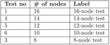
Table 5.2: Scalability of Hadoop cluster tests specification2
Test no # of nodes Label
1 16 16-node test
4 14 14-node test
5 12 12-node test
6 10 10-node test
3 8 8-node test
2
!"#$ %"$& '"!& #"&! %"$& (%")! $"'$ ($"*$ $"*! ($"'& (%"'& '("'&
&"*% ("%( &")! ("$* +"!& $"%! &"&& *"&& (&"&& (*"&& +&"&& +*"&& !&"&& !*"&& '&"&& '*"&&
(&,-. +&,-. (&,-. +&,-. (&,-. +&,-.
()/.0123425436 ()/.0123425437 %/.01234254
8 9: 2 3; : 9. <
82=>?2. 82=>50=4 82=>@>-91>42
(a) Time to complete
!"#$ %"$& '!"(& '#")# '#"*$ *'"*$ '"!' '"#) #"!& $"$$ )"$$ '$"$$ ')"$$ +$"$$ +)"$$ &$"$$ &)"$$ *$"$$ *)"$$
'(,-./01203214 '(,-./01203215 !,-./012032
6 78 0 19 8 7-:
60;<=0- 60;<3.;2 60;<><?7/<20
(b) Time to complete 20bln rows
!"!# !"!# !"!#
$%"&& $%"$&
$'"%!
(")! (")& (")&
&"&& *"&& (&"&& (*"&& $&"&& $*"&& !&"&&
(%+,-./01/2103 (%+,-./01/2104 )+,-./01/21
5 67 / 08 9 :
5/;<=/, 5/;<2-;1 5/;<><?6.<1/
(c) CPU time 10bln rows
!"!# !"$# !"!%
&'!"%% &'!"%%
&'%"%%
("(( ("(% ("$(
%"%% '%"%% )%"%% !%"%% *%"%% &%%"%% &'%"%% &)%"%%
&!+,-./01/2103 &!+,-./01/2104 *+,-./01/21
5 67 / 08 9 :
5/;<=/, 5/;<2-;1 5/;<><?6.<1/
(d) CPU time 20bln rows
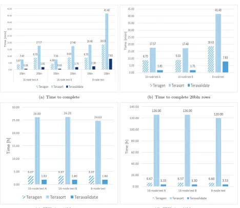
Fig. 5.1: Time to complete and CPU time for 16-node test A, 16-node test B and 8-node test
Similarly to test described in Sect. 5.1, the average of all three benchmarks for every result was taken as the most reliable value. As it can be seen in Fig. 5.2(a), which summaries the time to complete results for all five tests on both 10 and 20 bln rows, the scaling rises at half parabolic manner. The time to complete the
benchmarks gradually rises for both teragen sizes as more and more nodes are taken away from the cluster.
A simplified graph with the results only for 10 bln rows teragen size (cf. Fig. 5.2(b)) shows more clearly
how the results grow steadily but not linearly. The growth in case of teragen has progressed with a 17% rise
for 14-node test, 37% for 12-node test, 70% for 10-node test and 119% for 8-node test from the initial value in
test 1. Similar values were recorded forterasort: 13%, 37%, 78% and 146% respectively. In case ofteravalidate
the 14-node test and 12-node test have taken only 12% and 19% longer to complete than 16-node test. The remaining two tests however have taken 102% (10-node test) and 293% (8-node test) more time to run the benchmark.
The half parabolic growth tendency is also visible for the 20 bln rows generation and processing (cf.
!"#$ %"$& '"(! #")! )"'! **"'! ("$! *'"&! %"$& *%"(! $"'$ *$")$ %"'! +&"+$ *&"+! +'")& *!"!& !&"%! *%"'& '*"'&
&")% *"%* &"() +"($ &"(# !"*! *"*$ '"(& +"!& $"%! &"&& )"&& *&"&& *)"&& +&"&& +)"&& !&"&& !)"&& '&"&& ')"&&
*&,-. +&,-. *&,-. +&,-. *&,-. +&,-. *&,-. +&,-. *&,-. +&,-.
*(/.01234254 *'/.01234254 *+/.01234254 *&/.01234254 %/.01234254
6 78 2 39 8 7. :
62;<=2. 62;<50;4 62;<><-71<42
(a) Time to complete
!"#$ %"&! '"%! &"$! ("$) $"%$ ("%! *)"+! *!"!) *("%)
)"'( )"&' )"&# *"*$
+"!) )")) +")) %")) &")) (")) *)")) *+")) *%")) *&")) *(")) +)"))
*&,-./01 *%,-./01 *+,-./01 *),-./01 (,-./01
2 34 0 ,5 4 3-6
207890- 20781.7: 2078;8<3/8:0
(b) Time to complete 10bln rows
!"#$ %"&' ((")' ()"$' (!"*' (#"&# +$"+# +)"&$ '$"!' )(")$
("!( +"*# '"('
)"*$ #"!' $"$$ &"$$ ($"$$ (&"$$ +$"$$ +&"$$ '$"$$ '&"$$ )$"$$ )&"$$
(*,-./01 (),-./01 (+,-./01 ($,-./01 !,-./01
2 34 0 ,5 4 3-6
207890- 20781.7: 2078;8<3/8:0
(c) Time to complete 20bln rows
!"!# !"!# !"$% !"&# !"!#
'&"%% '&"(# '&"%! '&")!
'*"&!
("+! ("+( ("+* ("++ ("+%
%"%% $"%% (%"%% ($"%% '%"%% '$"%% !%"%%
(&,-./01 (*,-./01 (',-./01 (%,-./01 +,-./01
2 34 0 ,5 4 3-6
207890- 20781.7: 2078;8<3/8:0
(d) CPU time 10bln rows
!"!# !"#$ #"%$ #"&$ !"!%
'(!"%% '(!"%% '$%"%% '$("%%
'(%"%%
$"$$ $"&% $")# $"#% $")$
%"%% (%"%% &%"%% !%"%% *%"%% '%%"%% '(%"%% '&%"%%
'!+,-./0 '&+,-./0 '(+,-./0 '%+,-./0 *+,-./0
1 23 / +4 3 2, 5
1/678/, 1/670-69 1/67:7;2.79/
(e) CPU time 20bln rows
compared to the results of 10 bln tests. The changes in the teravalidate benchmark are more dramatic with 48% growth in 14-node test, 72% in 12-node test, 154% in 10-node test and 333% in 8-node test compared to 16-node test.
Similarly to the experiments of Sect. 5.2 the CPU time did not exhibit major fluctuations (cf. Figs. 5.2(d) and 5.2(e)).
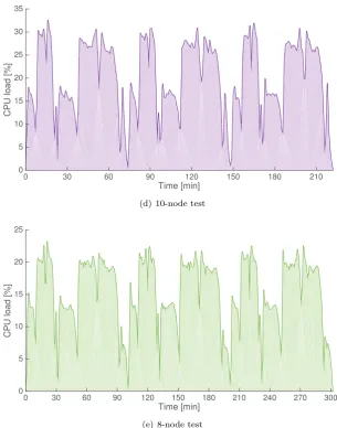
During the tests we have also observed that the cluster CPU utilisation3
was gradually dropping as the subsequent nodes were taken away to process the workload. In the 16-node test peaks were fluctuating around the 55% mark, with a maximum of 56.57% as shown in Fig. 5.3(a).
In the 14-node test, with just two nodes less that number came down to about 45% with a peak at 46.82% (cf. Fig. 5.3(b)).
The cluster with another 2 nodes removed in 12-node test (cf. Fig. 5.3(c)) brought down the CPU utilisation to about 40% (peak at 40.78%).
In test 6 with 10 nodes the cluster CPU utilisation drops to about 30% reaching up to 32.61% at its highest (cf. Fig. 5.3(d)).
In the 8 node test (cf. Fig. 5.3(e)) the CPU utilisation stays just above 20% with peak utilisation of 23.25%. Throughout the testing we have kept a close eye on the Disk Latency of the drives on the utilised cluster. Disk latency constitutes the amount of time that the hard drive takes to write a chunk of data. It has transpired that there are some serious constraints on the existing system. The lower the number of nodes processing the workload, the higher the latency of the drives. In 16-node test the nodes were scoring a latency of up to 3.4 seconds which is still a relatively high waiting time. However, as the tests progressed the bottleneck of drive latency was becoming more apparent. The latency in 14-node test reached 12 seconds at its highest, in 12-node and 10-node tests - about 18 seconds and as much as 57 seconds in the last test on 8 nodes (cf. Fig. 5.3).
6. Analysis and discussion.
6.1. Scaling beyond one rack. Running theterasort benchmark on the cluster has shown that there is
no major difference between the results on a single cluster deploying 16 nodes and two clusters with 8 nodes each. While it would be intuitive to assume that it would consume some overhead to communicate between the racks, it appears that if properly installed and configured the split racks do not make a large difference.
In the case of this study, the first stage of benchmarking - teragen - generates the data on both clusters
simultaneously and it is distributed evenly. This is due to the design of Job Tracker, which is a built-in service in Hadoop that oversees and manages the MapReduce jobs on the platform. It consults the Name Node to find out which Data nodes hold the necessary files to process a task. Job Tracker will always attempt to fetch the data from a local node from the same rack. Only when that is not possible the Name Node will refer it outside of the rack, reducing the overheads as a result.
A situation where this might prove not to be true is a cluster that is not balanced. ‘Balanced cluster’ is a term describing a situation where the data is evenly distributed across all nodes in all the racks. In a situation where a company has a successfully running cluster to which they add an additional rack in order to expand their Hadoop platform, they end up unbalancing the system. The data stays on the old rack and the new one remains empty. This often results in underutilisation of HDFS as the MapReduce tasks are not going to be scheduled on the added nodes unless the pre-existing racks are too busy to take new jobs. Also, the platform will experience larger network bandwidth consumption and slower job completions. In cases where the new nodes are assigned MapReduce tasks that they do not have data to complete, the files will have to be carried across the network, ultimately negatively impacting the performance.
In case of the two racks used for our testing, all the data has been generated on both racks evenly and we know that the cluster is balanced. The test results have proven that a Hadoop cluster if correctly designed does not lose on the performance when configured into more than one rack.
The testing also revealed that if we halved the amount of nodes processing the workload, the time to complete
have increased by more than 100% on all three benchmarks while running both teragen sizes. Intuitively, the
performance drop should stay just short of 100% as we are reducing the amount of nodes by half and there should be some loss of performance due to overheads for split rack.
3
Time [min]
0 30 60 90 120
C
PU
l
o
a
d
[
%
]
0 10 20 30 40 50 60
(a) 16-node test
Time [min]
0 30 60 90 120
C
PU
l
o
a
d
[
%
]
0 5 10 15 20 25 30 35 40 45 50
(b) 14-node test
Time [min]
0 30 60 90 120 150
C
PU
l
o
a
d
[
%
]
0 5 10 15 20 25 30 35 40 45
Time [min]
0 30 60 90 120 150 180 210
C
PU
l
o
a
d
[
%
]
0 5 10 15 20 25 30 35
(d) 10-node test
Time [min]
0 30 60 90 120 150 180 210 240 270 300
C
PU
l
o
a
d
[
%
]
0 5 10 15 20 25
(e) 8-node test
Fig. 5.3: Cluster CPU utilisation
The marginal difference in the results between tests 16-node-Aand16-node-B have proven that the
over-heads on a split rack are practically non-existent and the communication between the racks has a very minimal impact on the performance. That however does not explain the over 100% increase in time to complete.
The explanation of the drastic performance difference lies with theinodes(or index nodes). Inodein a
Unix-style files system is a data structure that keeps the contents of the file separate from the information stored
about the file. So for every file on the system there is a corresponding inode with a uniqueinode number [8].
Running close to the limit ofinodes explains the excessive time to complete not only on the smaller cluster
in 8-node test but also explains why duration of benchmarks more than doubles for 10 bln rows and 20 bln
rows. The amount of inodes and the space reserved for them is set during the creation of the file system. If
there are a lot of small files created on the disk, like in our case during testing, the system starts to run out
of inodes and drastically slows down long before it runs out of storage. This unfortunately cannot be changed
dynamically without re-formatting the drives. If the drives run out of inodes, no more files can be created on
the drives. This is why it is critical to accommodate for enoughinodes to successfully complete the workload
6.2. Scalability of Hadoop cluster. During the benchmarking of the Hadoop cluster we have observed
a gradual rise in time to complete on all three elements of the terasort benchmark. As the amount of nodes
drops, the time the platform requires to complete the process rises in a regular and predictable manner. Also the analysis of the Cluster CPU activity clearly tells us that the smaller the node count the less the processor capacity is utilised. With the highest number of nodes in our test - 16 - we only managed to use just over half of the cluster CPU potential. By halving the amount of nodes we are only using as little as 20% of total capacity. The 150% increase in utilization in case of 16 node cluster compared to 8 is dictated by the increased seek time on hard drives. Because the benchmarks are taking longer to complete, the stress on CPU is decreases as shown on figure 5.3, ultimately leading to underutilisation.
That activity very closely links to the Disk Latency already mentioned in Sect. 5.2, a hard drive consists of moving mechanical parts, some of the more important ones include platter, where the data is written, spindle that spins the platter, heads which write and read the data to/from the platter and is attached to the arm
that moves the head to the right spot on the platter. Inodes can be treated as logical cells that have a space
assigned on the platter. Those spaces are allocated during hard drive formatting and cannot be altered. As the
head writes the data to the platter, theinodes become assigned to each file on the drive. When there is a large
amount of small files created on the drive the inodes run out and the system cannot save any more data. As
the drive exhausts the inodes available, the seek time to write the data is extending. It takes more and more
time to find a freeinode and only then a file can be assigned to it (written). We can see that clearly in Fig. 6.1.
According to Microsoft and Oracle an acceptable disk latency in the industry should not exceed 10 ms [6]. In the best case scenario on a 16 node cluster we are experiencing as much as 3 seconds of latency on the disks. It exceeds the industry desired standards three hundred times. In comparison, for the 8 node cluster the latency is up to 57 seconds. It is clear that is a major cause of bottlenecks.
7. Conclusions and future work. In this paper we have explored two case scenarios where the hardware
configuration plays a large role in the performance of the cluster and will have an impact on the Big Data analytics workloads. In the first part we have established that as long as the data is evenly balanced across all the racks that make up the Hadoop platform, there are minimal overheads to accommodate the split racks. The corporations that decide to expand their Big Data environment have to remember to make use of balancing utilities to achieve that goal – otherwise the result will not reflect our findings.
During the testing process it transpired that the disk latency may cause high impact constraints. These constraints negatively impacted the duration of testing as well as utilisation of resources. In some cases we have experienced in excess of 200% or 300% increase in time required to complete benchmarks where we were expecting about 100% as we were either doubling the workload or halving the amount of resources. What we also have to keep in mind is that the testing conducted was a relatively small scale compared to what some large
scale corporations deploy; their workloads also are considerably larger than theterasort benchmark. The hard
drive seek time delays in those larger deployments may cause even bigger gap between the expected performance and what they actually achieve.
We have also found that the more the system is required to focus on seeking the inodes on the drives,
the less it focusses on processing the workload. This, combined with lower amount of nodes, ultimately leads to lower cluster CPU utilization. It is a large financial commitment for an origination to invest in hardware, especially enterprise class hardware. It is in their best interest to make sure that those resources are used to the best of their capabilities. That is why it is important that the corporation accurately assess the size and purpose of the Hadoop platform in order to correctly choose the required size of the cluster and also invest time to optimally configure it and test for bottlenecks.
There is yet a lot to explore in the domain of Hadoop optimisation. Although we have investigated the implications of different deployment scenarios and have found answers to our questions we also have found that the CPU time on the smallest 8-node cluster was shorter than on the larger ones. As the focus of this study was biased more towards the duration of the benchmarking, this issue has not been given much attention. Future analysis of the problem from the CPU side might give us more insight into other potential bottlenecks. Also the benchmarking on larger scale clusters with more variety of benchmark suites may unveil larger performance gap in the duration of the benchmarking as well as the CPU time.
Time [min]
0 20 40 60 80 100 120
L
a
te
n
cy
[ms]
0 500 1000 1500 2000 2500 3000 3500
(a) 16-node test
Time [min]
0 20 40 60 80 100 120 140 160
L
a
te
n
cy
[ms]
0 2000 4000 6000 8000 10000 12000 14000 16000 18000 20000
(b) 12-node test
Time [min]
0 50 100 150 200 250 300
L
a
te
n
cy
[s]
0 10 20 30 40 50 60
we would like to explore the power consumption dependence on various factors such as deployment model, configuration or number of nodes.
Also the investigation of networking choices and their impact would link to this study as the performance may be affected by the connectivity choices on the platform. Hence we plan to look into upgrading the cluster to InfiniBand in the future and present the difference in performance.
Acknowledgements. We gratefully acknowledge the support from of Mr. S. G. Anderson, Big Data
Solutions Engineer who has enabled the benchmarking process to take place at the Cloud and Big Data lab of the Client.
REFERENCES
[1] D. Altman, D. Machin, T. Bryant, and M. Gardner, Statistics with confidence: confidence intervals and statistical guidelines, John Wiley & Sons, 2006
[2] R. Appuswamy, C. Gkantsidis, D. Narayanan, O. Hodson and A. Rowstron,Scale-up vs scale-out for Hadoop: time to rethink?, Proceeding SOCC ’13 Proceedings of the 4th annual Symposium on Cloud Computing Article No. 20, 2013. [3] J. Dean, S. Ghemawat,MapReduce: Simplified Data Processing on Large Clusters, Communications of the ACM - 50th
anniversary issue 51 (1), 2008, pp. 107-113
[4] B. Hedlund,Understanding Hadoop Clusters and the Network, tech. report, 2011, http://bradhedlund.com/2011/09/10/ understanding-hadoop-clusters-and-the-network
[5] Hortonworks, Cluster Planning Guide, tech. report, 2013, http://docs.hortonworks.com/HDPDocuments/HDP1/HDP-1.3.0/bk cluster-planning-guide/bk cluster-planning-guide-20130528.pdf
[6] E. Markovich,Whats An Acceptable I/O Latency?, tech. report, Kaminario, 2010, http://kaminario.com/blog/whats-an-acceptable-io-latency/
[7] A. Nadkarni, Trends in Enterprise Hadoop Deployments, tech. report, IDC, 2013, http://www.avnetweb.com/comms/ avnet/redhat/liberate/resources/Trends in Enterprise Hadoop Deployments.pdf
[8] E. Nemeth,UNIX and Linux system administration handbook, Pearson Education, 2011.
[9] M. G. Noll, Benchmarking and Stress Testing an Hadoop Cluster With TeraSort, TestDFSIO & Co., 2011, http://www.michael-noll.com/blog/2011/04/09/benchmarking-and-stress-testing-an-hadoop-cluster-with-terasort-testdfsio-nnbench-mrbench
[10] N. Rouda, Achieving Flexible Scalability of Hadoop to Meet Enterprise Workload Requirements, tech. report, Enterprise Strategy Group, 2014, http://www.emc.com/collateral/analyst-reports/esg-emc-achieving-flexible-scaling-hadoop.pdf [11] E. Sammer,Hadoop operations, O’Reilly Media, Inc., 2012.
[12] M. Sevilla, I. Nassi, K. Ioannidou, S. Brandt and C. Maltzahn,A framework for an in-depth comparison of scale-up and scale-out, DISCS-2013 Proceedings of the 2013 International Workshop on Data-Intensive Scalable Computing Systems, pp. 13-18
[13] M. E. Wendt,Cloud-based Hadoop Deployments: Benefits and Considerations, tech. report, Accenture Technology Labs,
2014. https://www.accenture.com/t00010101T000000 w /jp-ja/ acnmedia/Accenture/Conversion-Assets/DotCom/
Documents/Local/ja-jp/PDF 2/Accenture-Cloud-Based-Hadoop-Deployments-Benefits-and-Considerations.pdf [14] T. White,Hadoop: The definitive guide, O’Reilly Media, Inc., 2012.
[15] C. Wilson,Who’s Using Hadoop and What are They Using It For?, 2015, http://blog.syncsort.com/2015/06/whos-using-hadoop-and-what-are-they-using-it-for
Edited by: Dana Petcu
Received: July 10, 2015