Some Discriminant-Based PAC Algorithms

Some Discriminant-Based PAC Algorithms

Paul W. Goldberg [email protected]

Department of Computer Science University of Warwick

Coventry, CV4 7AL, UK

Editor: Dana Ron

Abstract

A classical approach in multi-class pattern classification is the following. Estimate the probability distributions that generated the observations for each label class, and then label new instances by applying the Bayes classifier to the estimated distributions. That approach provides more useful information than just a class label; it also provides estimates of the conditional distribution of class labels, in situations where there is class overlap.

We would like to know whether it is harder to build accurate classifiers via this approach, than by techniques that may process all data with distinct labels together. In this paper we make that question precise by considering it in the context of PAC learnability. We propose two restrictions on the PAC learning framework that are intended to correspond with the above approach, and consider their relationship with standard PAC learning. Our main restriction of interest leads to some interesting algorithms that show that the restriction is not stronger (more restrictive) than various other well-known restrictions on PAC learning. An alternative slightly milder restriction turns out to be almost equivalent to unrestricted PAC learning.

Keywords: computational learning theory, computational complexity, pattern classification

1. Introduction

We present some PAC learning algorithms for various learning problems, within a new restriction of the PAC setting. We begin by explaining the motivation for studying the new restriction, and continue with some general results about it, followed by the algorithms.

1.1 Background and Motivation

A standard approach to classification problems (see for example (Duda and Hart, 1973), page 17) is the following. For each class, find a discriminant function that maps elements of the input domain to real values. These functions can be used to label any element x of the domain with the class label whose associated discriminant function takes the largest value on x. The discriminant functions are usually estimates of the probability densities of points in each class, weighted by the class prior (relative frequency of that class), in which case we are using the Bayes classifier.

giving lower bounds on sample-size or computational requirements. These results allow different models of the learning process to be provably distinguished from each other, in terms of the learning problems that are tractable within each model.

Most recent work on pattern classification (for example work on support vectors (Cristianini and Shawe-Taylor, 2000)) of course does not try to learn label class distributions, but rather to find decision boundaries that optimize some performance guarantee, usually misclassification rate. Performance guarantees are derived from observed classification performance in conjunction with other features of the boundary such as syntactic or combinatorial complexity, or the number of support vectors and margin of separation. The general approach clearly requires examples with different labels to be taken in conjunction with each other when finding a decision boundary. By contrast, discriminant functions are constructed from individual label classes in isolation. It seems clearly “easier” to find a good classifier by considering all data together (so as to apply empirical risk minimisation), than by insisting that each label class must be independently converted into a discriminant function. Noting Vapnik’s observation ((Vapnik, 2000), page 30) that one should not try to solve a problem via solving a more general problem, why exactly would we want to estimate the distributions of label classes?

The answer is that when the distributions can be found, the extra information that is obtained is often very useful in practice. In contrast with decision boundaries, we obtain for a domain element

x, the values of the probability densities of label classes at x, which provide a conditional

distri-bution over the class label of x. A predicted class label for x can then take into account variable misclassification penalties, or changes in the assumed class priors. There are of course other ways to obtain such distributions, for example using logistic regression, or more generally (for k-class classification) neural networks with k real-valued outputs re-scaled using the softmax activation function (see (Bishop, 1995) for details). However, unsupervised learning for each class—if it can be done successfully—has other advantages over these techniques, such as the following.

1. Label classes can be added without re-training the system. So for example if a new symbol were added to a character set, then given a good estimate of the probability distribution over images of the new symbol, this can be used in conjunction with pre-existing models for how the other symbols are generated.

2. Outlying instances are those that lie in regions of the domain where the distributions have low weight. We usually cannot assign a sensible label to such instances, however they may at least be recognised as a result of all class label distributions having very small weight around such an instance.

3. For applications such as handwritten digit recognition, it is arguably more natural—from the perspective of cognitive modeling—to model the data generation process in terms of 10 separate probability distributions, than as a collection of thresholds between different digits. This is because a handwritten zero (say) is nearly always the result of a process that first chooses the label “0” and then creates the image. It is not the result of a process that first generates a character and then assigns it the label “0” based on context, appearance or other criteria.

using multiple 2-class classifiers. How to combine them is a challenging topic that has itself re-ceived much recent attention, see for example (Guruswami and Sahai, 1999; Allwein et al., 2000). In practical studies such as (Platt et al., 2000) that build a multi-class classifier from a collection of 2-class classifiers, a distinction is made between separating each class from the union of the others (1-v-r classifiers, where 1-v-r stands for one-versus-rest) and pairwise separation (1-v-1 classifiers). Neither is entirely satisfactory—for example it may be possible to perform linear 1-v-1 separation for all pairs of classes, but not linear 1-v-r separation, while 1-v-1 classification (as studied in (Platt et al., 2000)) raises the problem of combining the collection of pairwise classifiers in a principled way to get an overall classification, for example ensuring that all classes are treated the same way. In (Platt et al., 2000), the first test for any unlabeled input is to apply the separator that distinguishes 0 from 9. Thus 0 and 9 are being treated differently from other digits (which in turn are also treated differently from each other.)

With regard to PAC learning, the approach of applying unsupervised learning to each label class, can treat situations where class overlap occurs (as is usually the case in practice). Standard PAC algorithms do not address this problem (although there have been extensions such as “probabilistic concepts” (Kearns and Schapire, 1994) that do so, and methods using support vectors that also allow decision boundaries that do not necessarily agree with all observed data). It is not hard to verify (see (Palmer and Goldberg, 2005)) that when we have good estimates of the class label distributions (in a sense described below in Section 1.3) then the associated classifier is approximately optimal in the agnostic PAC sense. For large data set sizes, it becomes feasible to find good estimates of these distributions, and obtain this more useful “summary” of the data.

The algorithms described in this paper are given in the context of simple 2-class classification, as opposed to multi-class classification. This is because we aim to explore the problems arising from an insistence upon treating each label class independently. The algorithms would however apply in a multi-class context where each pair of classes is separated by a boundary belonging to the given set of boundaries.

1.2 Formal Definition of the Learning Framework

In PAC learning (see for example (Anthony and Biggs, 1992) for a detailed introduction) there is a source of data consisting of instances generated by a probability distribution D over a domain X , labeled using an unknown “target function” t : X _{−→ {}0,1_}. The objective is to find a classifier

h : X_{−→ {}0,1_}which is a good approximation to t with respect to probability measure D. As usual we will letεdenote a misclassification rate (probability that t and h disagree on random x) andδ denote the uncertainty (probability that error rate εis not attained). We refer to the members of

t−1_{(1)as the “positive examples” and the members of t}−1_{(0)as the “negative examples”.}

Notation. For`<sub>∈ {</sub>0,1}let D`denote the restriction of D to t−1(`). Let p` denote the class prior for label`, p`=Prx_∼D(t(x) =`). We assume throughout that p`>0. Thus

Prx∼D`(x) = 1

p`Prx∼D(x) for t(x) =` Prx∼D`(x) =0 for t(x) =1−`

For any probability distribution P over X (for example D or D`), an algorithm with access to P may in unit time draw an unlabeled sample from P.

It is shown in (Haussler et al., 1991) that the standard PAC framework is equivalent to a “two-button” version, where an algorithm has access to a “positive example oracle” and a “negative example oracle”. (The two-button version conceals the class priors and only gives the algorithm access to the distribution as restricted to each class label. Thus the oracles generate examples from

D1and D0respectively.) We define a restriction of “two-button” learning as follows.

Definition 1 Suppose algorithm

A

has access to a distribution P over X , and the output of

A

is a function f : X _−→IR. Execute

A

twice, using D1(respectively D0) for P. Let f1and f0be the

functions obtained respectively. For x_∈X let

h(x) =1 if f1(x)> f0(x)

h(x) =0 if f1(x)< f0(x)

h(x)undefined if f1(x) = f0(x)

If

A

takes time polynomial inε−1andδ−1, and h is PAC with respect toεandδ, then we will say that

A

PAC-learns via discriminant functions.

It is clear that if

A

can be found such that the resulting h is PAC, then we have PAC learnability in the two-button setting, and hence standard PAC learnability.

In specifying the restriction above, we are keeping it both simple and “severe”, in the sense of making it difficult to find algorithms within the restricted framework. This is with a view to getting strong positive results, and also to maximizing the potential for negative results (PAC learnable problems that are hard within the restricted setting). One could devise less severe restrictions to capture the general idea of learning via discriminant functions. Alternatives are discussed at the end of this section.

We also consider the following slightly less severe variant related to POSEX learnability as

introduced in (Denis, 1998), in which

A

has access to D (in (Denis, 1998) the “EX” oracle), in

addition to D1(in (Denis, 1998) the “POS” oracle). This is formalized as Definition 2, and it turns out that we can be much more specific about learnability in this sense, namely it is intermediate between PAC learnability with uniform misclassification noise and basic PAC learnability.

Definition 2 Suppose algorithm

A

has access to D in addition to distribution P over X , and the output of

A

is a function f : X _−→IR. Execute

A

twice, using D1(respectively D0) for P. Let f1

and f0be the functions obtained respectively. For x∈X let

h(x) =1 if f1(x)> f0(x)

h(x) =0 if f1(x)< f0(x)

h(x)undefined if f1(x) = f0(x)

POSEX learnability requires that f1be a 0/1-valued function that constitutes a PAC hypothesis. We discuss the relationship in more detail in the next section.

Notation. We refer to the two instances of the unsupervised learning algorithm as

A

₁ and

A

₀, so that

A

₁consists of

A

with the (unlabeled) positive data as input, and

A

₀is

A

with the (unlabeled) negative data as input. (Note however that learning according to Definition 1 or 2 does not allow

A

<sub>`</sub> to use the value of`.) We let S`denote the sample of unlabeled data drawn by

A

`.

Let us conclude this section by considering alternative restrictions to PAC learnability that cap-ture the informal notion of learning via discriminant functions. We could for example ask that f1 and f0should be probability distributions. Our reason for not doing so is that, while we believe that the functions produced by our algorithms can be re-scaled on an ad-hoc basis to become probability distributions, there is no guarantee in the distribution-free PAC setting that they are similar to the unknown distributions D1and D0.

Another natural candidate is a variant in which

A

₁ and

A

₀ are two distinct agents that know their class labels. Equivalently, we would be seeking two algorithms

A

₁ and

A

₀ that respectively have access to the positive and negative data (equivalently, an algorithm

A

<sub>`</sub>that may use the value `). Observe however that this relaxation is not helpful for any concept class

C

that is closed under complement (meaning that for all c_∈

C

, we also have X_\c_∈

C

). Consequently, any algorithms that require this relaxation would need to exploit additional prior information about data from different classes. There’s nothing wrong with that of course, but it departs from our focus on the approach of independently processing each label class.

1.3 Related Work

There has been much work on the comparison of alternative notions of PAC learning with each other, with the criterion for distinguishability being that some learning task (concept class) should be tractable1 in one variant but not in the other. The early paper of (Haussler et al., 1991) showed that various alternative definitions of PAC learnability are equivalent in this sense. Examples of distinctions that have been found between different restrictions to the framework include learning with a restricted focus of attention (Ben-David and Dichterman, 1998, 1994) which is shown to be more severe that learnability in the presence of uniform misclassification noise. Learnability with Statistical Queries (Kearns, 1998) is also known to be at least as severe as learnability with uniform misclassification noise. Perhaps the most important result of this kind is the equivalence between PAC learnability and “weak” PAC learnability found by (Schapire, 1990) which led to the development of boosting techniques. The paper (Blum, 1994) exhibits a concept class that distinguishes PAC learnability from mistake-bound learning, and that is of interest here since we use the same concept class (in Section 3.3) to show that our restriction of PAC learnability is likewise distinct from mistake-bound learnability.

We noted that learning under the constraint of Definition 2 is related to POSEX learning. Specif-ically we have:

Observation 1 If a concept class and its complement are POSEX learnable, then they are learnable

under Definition 2.

Proof (sketch; the following technique is used in more detail in Theorem 4) Let

A

_P be a POSEX algorithm for

C

and let

A

0

P be a POSEX algorithm for

C

0, the class of sets whose complements are

members of

C

. An algorithm

A

in the sense of Definition 2 works as follows.

A

can sample from

D, and it uses samples from D`as “positive” examples.

A

applies

A

P and

A

P0 to this data, and at

least one of the two hypotheses h,h0 is PAC, since the “positive” data really is positive from the perspective of one of

A

_Pand

A

0

P.

h and h0are then tested on further data; the chosen hypothesis should contain almost all samples from D`, and if both h and h0 do so, choose the one that contains fewer samples from D. That hypothesis with high probability maps samples from D`to 1 and samples from D1−`to 0. Let

A

1 and

A

₀ be the two runs of

A

having access to D1 and D0 respectively. The overall hypothesis is obtained from two functions found by

A

₁ and

A

₀, and its misclassification rate is at most the sum of their error rates.

In Section 2 we show that if a concept class is learnable in the presence of noise, then it and its complement are POSEX learnable, and hence by the above observation, learnable under Defini-tion 2. The result of SecDefini-tion 2 answers a quesDefini-tion raised by (Letouzey et al., 2000) (the hierarchies of inclusions given in Equations (4,5) of (Letouzey et al., 2000) can be merged).

There are some interesting algorithms having PAC-like performance guarantees for learning probability distributions; the topic was introduced in (Kearns et al., 1994), see also (Cryan et al., 2001; Freund and Mansour, 1999; Frieze et al., 1996; Dasgupta, 1999). The criterion for learning a distribution D is to obtain a hypothesis distribution which is withinεof D under some measure of similarity. The KL distance and the variation distance are usually considered. We noted above that when distributions are learned under these criteria, the Bayes classifier achieves agnostic PAC-ness. However, the algorithms we describe here differ substantially from these previous ones (as well as from the algorithms in the much more extensive general literature on unsupervised learning). The reason is that our aim is not really to approximate a distribution over inputs. Rather, it is to construct a discriminant function in such a way that we expect it to work well in conjunction with the corresponding discriminant function constructed on data with the opposite class label.

1.4 Summary of Results

The rest of the paper is organized as follows. In Section 2 we consider learning under Definition 2 in which

A

<sub>`</sub>has access to D in addition to D`. We show that PAC learnability with uniform misclas-sification noise implies PAC learnability with discriminant functions and access to D. This gives us a good understanding of how learning under Definition 2 fits in with other restrictions.

In Section 3 we move to the trickier issue of learning according to Definition 1. We exhibit algorithms that show that the restriction is not more severe than various other restrictions of PAC learning. In Section 3.1 we show that parity functions are learnable in this setting, which dis-tinguishes it from learnability in the presence of noise (subject to the “noisy parity assumption”, which is the widespread assumption that parity functions are hard to learn in the presence of uni-form misclassification noise) as well as Statistical Query (SQ) learnability (Kearns, 1998) (since it is known from (Kearns, 1998) that parity functions are not learnable using SQs.) In Section 3.2 we distinguish the setting from learnability from positive data only (or negative data only) by study-ing the class of unions of intervals on the real line. In Section 3.3 we diststudy-inguish the settstudy-ing from mistake-bound learning, using a concept class from (Blum, 1994).

that we have not been able to extend to three or more dimensions. In Section 3.5 we show how to learn monomials provided that the input distribution D is an unknown product distribution. Learn-ing under this sort of assumption is in a sense intermediate between learnLearn-ing with access to D (Definition 2) and learning via discriminant functions in the sense of Definition 1.

2. Learning via Discriminant Functions with Access to D

In this section we show that given a standard noise-tolerant PAC learning algorithm, we may use it to construct an algorithm for POSEX learning and hence learning in the restriction of Definition 2. We do this in two stages—Proposition 3 shows how this is achieved provided that an estimate of the class prior p` is provided to

A

`, and Theorem 4 extends the result to the setting in which the class priors are unknown.

Here is an overview of the proofs in this section. Proposition 3 analyses learning with a given noise rate. This uses a standard definition of noise-tolerant PAC learning in which an algorithm

A

η has parameterη. ηis the probability that an example is mislabeled; 0_≤η<1

2.

A

ηshould then be polynomial in(1

2−η)−1 in addition to other parameters. Given the class prior p` (the probability that a random instance has label`) we can generate random samples from a fixed distribution that is a mixture of D and D`, such that they have uniform misclassification rate, which allows

A

ηto be used. In fact, we show that an additive approximation p`can be used in place of p`. This is done by exhibiting a coupling of the two labeled sample distributions (one using p`and the other using p`), in which they are very likely to generate the same data.

In Theorem 4 we exploit the fact that an approximation p` can be used. The algorithm of

Figure 2 tries out a sequence of values for p`, at least one of which is a good approximation to p`. The previous algorithm is used for each of these values, which generates a collection of hypotheses, and the empirically best hypothesis is shown to be PAC.

Proposition 3 Let

A

ηbe an algorithm with parameterη, 0_≤η<1

2, that has access to labeled data,

where elements of X are distributed according to D, with a uniform label noise rate ofη. Suppose that

A

ηuses time p(ε−1_,δ−1_,(1

2−η)−

1_{)(where p is some polynomial), and with probability at least} 1₋δreturns a hypothesis having error at mostε(with respect to D).

For `<sub>∈ {</sub>0,1<sub>}</sub> let p`=Prx∼D(t(x) =`). Suppose that |p`−p`| ≤∆/p(ε−1,δ−1,(1₂−η)−1).

(∆_∈[0,1].) Suppose that the algorithm of Figure 1 is executed with input p`and access to D`and

D. Then with probability 1₋δ₋∆, the algorithm outputs f`: X−→ {0,1}satisfying

Pr_x∼1

2(D+D`)(f`(x)6=t(x))≤ε for `=1

Pr_x∼1

2(D+D`)(f`(x)6=1−t(x))≤ε for `=0

Comment. The fact that f`has error at mostεfor x∼ 1<sub>2</sub>(D+D`)implies that f`has error at most 2εfor x_∼D.

Proof We may assume that the concept class

C

is closed under complementation, since if

C

is learnable with misclassification noise then its closure under complementation is also learnable under misclassification noise.

Since

C

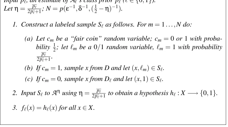
is closed under complementation, it suffices by symmetry to show that f1satisfies: with probability at least 1₋δ₋∆, Pr_x∼1

Input p`, an estimate of

A

`’s class prior p`(`∈ {0,1}).

Letη= p`

2p`+1; N=p(ε

−1_,δ−1_,(1

2−η)−1).

1. Construct a labeled sample S`as follows. For m=1. . . ,N do:

(a) Let cm be a “fair coin” random variable; cm=0 or 1 with

proba-bility 1₂; let`mbe a 0/1 random variable, `m=1 with probability p`

2p`+1.

(b) If cm=1, sample x from D and let(x, `m)∈S`.

(c) If cm=0, sample x from D`and let(x,1)∈S`.

2. Input S`to

A

ηusingη= _2pp<sub>`</sub>`₊₁ to obtain a hypothesis h`: X−→ {0,1}.

3. f`(x) =h`(x)for all x∈X .

Figure 1: Learning in the sense of Definition 2 using noise-tolerant PAC algorithm and estimates of class priors

Let(x,j)be the element of S1constructed on the m-th iteration.

Pr(t(x) =0) = Pr(cm=1)Prx∼D(t(x) =0) =1₂(1−p1) Pr(t(x) =1) = 1₋1₂(1₋p1) =1₂(1+p1)

(1)

Next we give expressions for misclassification rates Pr(j=0_|t(x) =1)and Pr(j=1_|t(x) =0). Consider first the case that t(x) =1. Note that

Pr(j=0_|t(x) =1) = Pr(j=0_|t(x) =1_∧cm=0)Pr(cm=0|t(x) =1)

+Pr(j=0_|t(x) =1_∧cm=1)Pr(cm=1|t(x) =1).

Pr(j=0_|t(x) =1_∧cm=0) =0, since if cm=0 then Step (1c) assigns label 1. Hence

Pr(j=0|t(x) =1) =Pr(j=0|t(x) =1∧cm=1)Pr(cm=1|t(x) =1). (2)

When cm=1, we have j=`mwhere`m=1 with probability p1/(2p1+1), so

Pr(j=0_|t(x) =1_∧cm=1) =1−

p1 2p1+1

= p1+1

2p1+1

. (3)

Pr(cm=1|t(x) =1) =

Pr(cm=1)Pr(t(x) =1|cm=1)

Pr(t(x) =1) =

1 2p1 Pr(t(x) =1).

Pr(t(x) =1) =1₂(1+p1)by Equation (1), hence

Pr(cm=1|t(x) =1) =

1 2p1 1

2(1+p1)

= p1

1+p1

Hence from Equations (2) and (3) and (4),

Pr(j=0|t(x) =1) = p1+1

2p1+1

_p1

1+p1

.

Now consider the case that t(x) =0 (where(x,j)is the labeled exampled constructed on the

m-th iteration of

A

1); note that

Pr(j=1_|t(x) =0) = Pr(j=1_|t(x) =0_∧cm=0)Pr(cm=0|t(x) =0)

+Pr(j=1_|t(x) =0_∧cm=1)Pr(cm=1|t(x) =0).

If cm=0 then from Step (1c), t(x) =1. Hence

Pr(cm=1|t(x) =0) = 1

Pr(cm=0|t(x) =0) = 0.

Consequently,

Pr(j=1|t(x) =0) =Pr(j=1|t(x) =0∧cm=1). (5)

When cm=1 we have j=`mwhere`m=1 with probability p1/(2p1+1), so

Pr(j=1_|t(x) =0_∧cm=1) =

p1

2p1+1. (6)

From (5) and (6),

Pr(j=1_|t(x) =0) = p1

2p1+1.

Based on the above expressions for the misclassification rates Pr(j=0_|t(x) =1)and Pr(j=

1 _|t(x) =0), and noting that N is defined in Figure 1, Step (1) of the algorithm of Figure 1 is equivalent to the following:

1. For m=1. . .N do:

(a) Sample x from the mixture1₂(D+D1). (b) Sample rmuniformly at random from[0,1].

(c) If t(x) =1, then if rm<(_2pp1₁+₊1₁)(₁₊p1_p1)label x incorrectly else label x correctly.

(d) If t(x) =0, then if rm<_2pp1₁₊₁ label x incorrectly else label x correctly.

Let DA be the above distribution over samples of size N. Let Dη be the following distribution

over samples of size N:

1. For m=1. . .N do:

(a) Sample x from the mixture1₂(D+D1). (b) Sample rmuniformly at random from[0,1].

Let SN denote the set of labeled samples of size N. Define a distribution D2N over SN×SN

by using the same sequence of x’s and rm and the above procedures for constructing the labeled

samples, so that the two marginal distributions over SN are DA and Dη. For(S,S0)∼D2N, Pr(S₆=S0)_≤N_· Pr

x∼1 2(D+D1)

(t(x) =1)_· p1+1

2p1+1

_p1

1+p1

− p1

2p1+1

.

This is because there are N opportunities for S to differ from S0, and this occurs when x sampled from1₂(D+D0)satisfies t(x) =1. In that case, the labels will differ when rmlies between_2pp1₁₊₁and

(_2pp1+1

1+1)( p1

1+p1). Consequently,

Pr(S₆=S0)_≤N_·|p1−p1(

1+p1

1+p1)|

2p1+1 ≤N·(2p1+1)

−1

· |p1−p1| ≤N|p1−p1|. By definition of

A

η, for S_∼Dη, N=p(ε−1_,δ−1_,(1

2−η)−1),η=

p1

2p1+1, with probability 1−δ,

A

ηon input S returns h0having error Pr(h0(x)₆=t(x))_≤εfor x_∼1₂(D+D1).

Hence for S_∼DA, N =p(ε−1,δ−1,(1₂−η)−1), with probability 1−δ−N(|p1−p1|),

A

η on input S returns h0 having error Pr(h0_{(x)6=t(x))≤εfor x∼} 1

2(D+D1). Given our assumption that

|p1−p1| ≤∆/N=∆/p(ε−1,δ−1,(1₂−η)−1), the result follows.

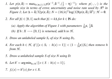
1. Let p(ε,δ) = max_0≤η≤1/3p(ε−1_,δ−1_,(1 2−η)−

1_{); where p(·,·,·) is the}

sample size in terms of error, uncertainty and noise rate used by

A

η in Figure 1; Let∆=δ/32p(ε,δ); N= (16/ε)2_{log(128p(ε,δ)/δ}2_);

_H

₌/0_.

2. For all p`∈[0,1]such that p`=k∆for k∈IN do:

(a) Apply the algorithm of Figure 1 with parameters ₁₆1ε, 1₄δ. (b) If h : X_{−→ {}0,1_}is returned, add h to

H

.

3. Draw an unlabeled sample S`of size N using D`.

4. For each h_∈

H

, if _|{x_∈S` : h(x) =1}|<(1−<sub>16</sub>3ε)|S`|then remove h

from

H

.

5. Draw a unlabeled sample S of size N using D.

6. Let h0=arg min_h∈H|{x∈S : h(x) =1}|.

7. f`(x) =h0(x)for x∈X .

Theorem 4 Let

A

ηbe a noise-tolerant algorithm as defined in Proposition 3.

For `<sub>∈ {</sub>0,1<sub>}</sub>, the Algorithm of Figure 2 given access to D` and D, with probability at least 1₋δ outputs (in polynomial time) f` with Prx∼D(f`(x)6=t(x))≤εfor `=1, and Prx∼D(f`(x)6= 1−t(x))_≤εfor`=0.

Comment. As a consequence we have learnability in the sense of Definition 2, since when we derive classifier h from f1and f0, the error of h is at most the sum of the errors of f1 and f0. (By the error of f0we mean the probability that f0(x)is not equal to 1−t(x).)

Proof LetPrbx∈S(π(x))denote the empirical probability that x satisfies propertyπ, with respect to

sample S. We show first that the expression for N used by the algorithm of Figure 2 guarantees that with probability at least 1₋1₂δ,

∀h_∈

H

Pr

x∼D`

(h(x) =1)₋Prbx∈S`(h(x) =1)

≤ 1

16ε (7)

∀h_∈

H

Pr

x∼D(h(x) =1)−Prbx∈S(h(x) =1)

≤₁₆1 ε (8)

We are asking that the relative frequencies (over N observations) of a set of at most 2_|

H

_|events should be within ₁₆1ε of their probabilities. Taking a union bound, it is sufficient that N should satisfy: Given any f : X _{−→ {}0,1_}, with probability at least 1₋δ/(4_|

H

_|)

Pr

x∼D(f(x) =1)−Prbx∈S(f(x) =1)

≤₁₆1 ε.

Recall Hoeffding’s inequality: Let Y1, . . . ,YN be Bernoulli trials with probability p of success.

Let T =Y1+. . .+YNdenote the total number of successes. Then forγ∈[0,1], Pr(|T−pN|>γN)≤

2e−2Nγ2.

This means that N is sufficiently large if N satisfiesδ/(4|

H

_|)_≥2e−2N(ε/16)2. Since|

H

_{| ≤}1/∆, it is sufficient for N to satisfyδ∆/4_≥2e−2N(ε/16)2.

For∆=δ/32p(ε,δ),

δ2_{/128p(ε,δ)≥2e}−2N(ε/16)2

The equation is satisfied by putting N= (16/ε)2_{·log(128p(ε,δ)/δ}2_{), polynomial in the parameters.} Assume that`=1. We assume as before that the concept class is closed under complementation, so that the proof for`=0 is similar but using the complement of t in place of t.

Note that the algorithm of Figure 1 constructs a noise rateηin the range[0,1

3]based on p`, so each application of Algorithm 1 in Step (2a) uses sample size at most p( 1

16ε− 1_,1

4δ−

1_{). (Polynomial}

p(_·,_·)is defined in Figure 2.)

One of the values of p` used in Step (2a) as input to Algorithm 1 satisfies|p`−p`|<∆. As a result, applying Proposition 3 we have that with probability 1₋1₂δ, there exists h∗_∈

H

satisfying

Pr

x∼1 2(D+D1)

(h∗(x)₆=t(x))_≤ 1

16ε.

We may deduce that

Prx_∼D1(h∗(x)6=t(x))≤1₈ε

Prx∼D(h∗(x)6=t(x))≤1₈ε.

(9)

1. for h∈

H

, if Prx∼D(h(x) =0∧t(x) =1)>1₄εthen h is eliminated in Step 4.

2. h∗is not eliminated in Step 4.

3. For h_∈

H

, if Prx∼D(h(x) =1∧t(x) =0)> 1₂εthen h is eliminated in Step 6.

Suppose that Prx∼D(h(x) =0∧t(x) =1)> 1₄ε. Then Prx∼D1(h(x) =0∧t(x) =1)> 1₄ε/p1≥ 1₄ε. Hence by (7),

b

Prx∈S1(h(x) =0∧t(x) =1)>

1 4ε−

1 16ε=

3 16ε. From (7) and (9),

b

Prx∈S1(h∗(x) =0∧t(x) =1)≤

1 8ε+

1 16ε=

3 16ε.

Hence Step 4 does not eliminate h∗but it eliminates all h with Prx∼D(h(x) =0∧t(x) =1)>1₄ε.

Now suppose that Prx_∼D(h00(x) =1∧t(x) =0)> 1₂εfor some h00∈

H

after Step 4. We have

just shown that h00satisfies Prx∼D(h00(x) =0∧t(x) =1)≤ 1₄ε. Consequently, Prx∼D(h00(x) =1)−

Prx∼D(t(x) =1)>1₂ε−1₄ε=₄1ε. Meanwhile note from (9) that Prx∼D(h∗(x) =1)−Prx∼D(t(x) =

1)_≤1₈ε. As a result, Prx_∼D(h00(x) =1)−Prx_∼D(h∗(x) =1)>1₄ε−1₈ε=1₈ε. From (8), b

Prx∈S(h00(x) =1)−Prbx∈S(h∗(x) =1)>0.

Hence h00is eliminated at Step 6.

Hence all h_∈

H

with error at leastεare eliminated with probability 1₋1₂δ. With probability at least 1−1

2δthere exists h∗∈

H

with error less thatε. Putting these together, with probability at least 1₋δwe are left with h0having error less thanε.

3. Learning via Discriminant Functions without Access to D

We exhibit algorithms that show that learnability in the sense of Definition 1 is distinct from various well-known restrictions of PAC learnability. We also study a special case of the problem of learning monomials (in which D is known to belong to a particular class of distributions), for which we have no algorithm in the distribution-independent setting.

Our algorithms are mostly proven to have the PAC property in a standard way, by arguing that the hypothesis is consistent with the data, and furthermore that it belongs to a class of hypotheses that have description length polynomial in the parameters of the problem, and sub-linear in the sample size. (This is the “Occam algorithm” property (Blumer et al., 1987)). For Sections 3.2 and 3.4 we use the (more generally applicable) Vapnik-Chervonenkis dimension (Blumer et al., 1989; Vapnik, 2000) of the class of hypotheses.

3.1 Parity Functions

The following result distinguishes our learning setting from learnability with uniform misclassifica-tion noise, or learnability with a restricted focus of attenmisclassifica-tion.

An instance is an element of_{0,1_}n_{, representing a sequence of values of n boolean variables. A}

parity function (Helmbold et al., 1992) has an associated subset of the variables, and an associated

Theorem 5 The class of parity functions is PAC learnable via discriminant functions. Proof Observe that the class is closed under complementation.

To learn a parity function from positive examples only, in an essentially similar way to the algo-rithm of (Helmbold et al., 1992),

A

_`finds the affine subspace of GF(2)n_{spanned by its examples,}

and f` assigns a value of 1 to elements of that subspace and a value of 0 to all other elements of the domain. (By “span” we mean with respect to GF(2)n_{, as opposed to IR}n_{. GF(2), the generic}

field with two elements 0 and 1, has addition modulo 2, so that the sum of two 0/1 vectors is their bitwise exclusive-or. Generally the positive examples of a parity function would span all of IRn.)

In more detail, let xi be the i-th entry of bit vector x. The positive examples of a parity function

satisfy∑_icixi=b (all addition and multiplication modulo 2), where ci,b∈GF(2). Let x0 be an

arbitrary positive example; positive examples x satisfy∑_ici(xi−x0i) =0, and negative examples do

not satisfy this. Hence, the subspace constructed by

A

₁ will be a subset of∑ici(xi−x0i) =0, and

will contain no negative examples.

A

₀constructs a subspace that contains all the negative data and no positive examples.

We have that f`(x) =0 for all x with t(x) =1−`, and f`(x) =1 for all x∈S` (the unlabeled sample obtained by

A

_`).

The overall hypothesis h has description length O(n2_{) (a spanning set has at most n vectors,} each of length n) and h is consistent with the training data; thus we have PAC-ness by the standard Occam-algorithm argument.

3.2 Unions of Intervals

Let X=IR, and let t : X_{−→ {}0,1_}be the indicator function of a union of k intervals in IR. We show that the class of all such functions, is learnable by discriminant functions in time polynomial in ε−1_,δ−1_{and k. A union of more than one interval cannot be PAC-learned from just positive or just} negative data, simply because it is impossible to guess where the data with the opposite label may lie. Learnability via discriminant functions is thus distinct from learnability from positive examples only, or from negative examples only.

Theorem 6 The class of unions of k intervals on the real line is learnable via discriminant

func-tions.

Proof Construct discriminant functions f0 and f1as follows. Given an (unlabeled) sample, and a point x_∈IR, our discriminant function maps x to the negation of its distance to its nearest neighbor in the sample. (Intuitively, it makes sense that x should get a higher value if it is close to a data point in the sample.) We show furthermore that this rule creates a classifier that is “simple” (a union of k intervals) and consistent with the data.

More precisely, given (unlabeled) sample S`⊂IR of size O(k log(δ−1ε−1)/ε), let dNN(x,S`) = minx`∈S`{|x−x`|}. Let f`(x) =−dNN(x,S`). Recall that h(x) =1 if f1(x)> f0(x) and h(x) =0 if

f1(x)< f0(x). We show that h is PAC.

For x,x0_∈S`, suppose x,x0belong to the same interval of t−1(`). Then[x,x0]⊆h−1(`), since any point between x and x0is closer to at least one of x or x0than to any point x00for which t(x00_)6=t(x).

and h(x) =0 for h constructed according to Definition 1. Similarly, for x∈(1

2(x0+x1),x1), h(x) =1.

h(1₂(x0+x1))is undefined.

For S0∪S1sorted in ascending order, there are at most 2k pairs of consecutive points x,x0in the sequence where t(x)₆=t(x0).

Hence h is undefined on at most 2k elements of IR, and h−1(1) is a union of at most k inter-vals, and h−1(0)is a union of at most k+1 intervals. The VC dimension of unions of k intervals is 2k, so using the results of (Blumer et al., 1987), the sample size required for PAC learning is

O(k log(δ−1_ε−1_)/ε).

Comment. This nearest-neighbour rule does not work in more than one dimension, given that the input distribution D is closen by an adversary. Suppose we wish to learn a linear threshold in the plane IR2. Suppose D is uniform over two parallel line segments that are very close but on opposite sides of the classification threshold. Then the probability is only about 1₂that the nearest neighbour of a data point x will have the same label as x. In Section 3.4 we show how to learn linear thresholds in the plane using a more sophisticated rule.

3.3 Distinguishing the Model from the Mistake-bound Setting

In (Blum, 1994), Blum exhibits a concept class that is PAC learnable, but is not (in polynomial time) learnable using membership and equivalence queries, assuming that one-way functions exist. In this section we show that the concept class is PAC learnable via discriminant functions in the sense of Definition 1. We review the concept class introduced in (Blum, 1994). Let X=_{0,1_}n_.

If A is a probabilistic polynomial-time algorithm that computes a function from_{0,1_}∗_to{0,1},

and g is some function from_{0,1_}∗to_{0,1_}∗, let

P

k(A,g(s))denote the probability that A(g(s)) =1

for strings s of length k generated uniformly at random.

Let G be a Cryptographically Strong Pseudorandom Bit (CSB) generator with stretch p(k) =2k. For polynomial p a CSB generator is defined as follows.

Definition 7 A deterministic polynomial-time program G is a CSB generator with stretch p if on

input s_{∈ {}0,1_}k it produces an output in_{0,1_}p(k)_{and for all probabilistic polynomial-time} algo-rithms A, for all polynomials Q, for sufficiently large k (k depending on A and Q),

|

P

_k(A,G(s))₋

P

_p(k)(A,s)_|< 1

Q(k).

Thus, no polynomial-time algorithm can distinguish between strings generated uniformly at random from_{0,1_}2k_{, and strings obtained by taking the output of G for a random input string of} length k. (Technically, the definition allows A to be a circuit family.)

For strings x and y, let x_◦y denote their concatenation. For a bit string x let LSB[x]denote the rightmost bit of x. Letλdenote the empty string. For bit string s of length k, G(s)is a bit string of length 2k, and we define the following notation.

1. Let G0(s)be the leftmost k bits of G(s).

2. Let G1(s)be the rightmost k bits of G(s).

4. Let G0₁(s) =λ.

5. If i=i1···id (where the ijare binary digits), let Gi(s) =Gid(Gid−1(···Gi1(s))).

The concept class is defined as follows:

Definition 8 Let k=_b√n_{c −}1 and let

C

=_{cs}s∈{0,1}kwhere c_sis defined as follows. • csis the indicator function of{xis : i∈ {0,1}kand LSB[Gi1_···ik(s)] =1}

where for i=i1···ik,

• xi_s=i_◦G0_i1(s)_◦G0_i2(Gi1(s))◦Gi30 (Gi1i2(s))◦. . .◦G0ik(Gi1···ik−1(s))◦0 w

where w is chosen to ensure that_|xi_s|=n.

Definition 8 is slightly different from the corresponding definition of (Blum, 1994), where k=_b√n_c. We use k=_b√n_{c −}1 so that the length of xi_sis always less that n, and we can then “pad it out” to a length of exactly n using the string 0won the right-hand side.

Note that for any fixed s, a bit string of length n of the form xi_s is determined entirely by i, its first k bits. We will let the index of a bit string of length n refer to its first k bits, viewed as a binary number (to give the natural ordering on indices). For a string x let index(x)denote this number, regardless of whether x is well-formed according to Definition 8. (If x is not well-formed,

x is a negative example of cs, i.e. cs(x) =0.) Algorithm Compute-Forward (Figure 3) shows how

to take any positive example xi_s, together with an index j>i, and construct the pair_hxsj,cs(xsj)iin

polynomial time.

The following notation is used in Algorithm Compute-Forward:

1. Let zi_sbe the correctly labeled example_hxi_s,cs(xis)i.

2. Let zi

sbe the incorrectly labeled examplehxis,1−cs(xis)i.

3. For i1, . . . ,id∈ {0,1}d, let Gi1···id(s) =G0i1(s)◦Gi20 (Gi1(s))◦. . .◦G0id(Gi1···id−1(s)).

So xi_s=i_◦Gi1···ik_(s)◦0w_.

From (Blum, 1994) we know that

C

is not learnable (in time polynomial in n) in the mistake-bound model. We review the PAC learning algorithm of (Blum, 1994) and show how to adapt it to the constraint of Definition 1.

We noted that Algorithm Compute-Forward, given a positive example xi_sand j>i, produces a

correctly-labeled examplehxsj,cs(xsj)i. Based on this observation, we assign values to examples as

shown in Figure 4.

Theorem 9 The concept class of (Blum, 1994) is learnable via discriminant functions. Proof We use the algorithm of Figure 4 to construct discriminant functions.

Recall that for x_{∈ {}0,1_}n_{, index(x)denotes the k bit binary number forming a prefix of x, for}

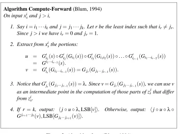
Algorithm Compute-Forward (Blum, 1994)

On input xi_sand j>i,

1. Say i=i1···ikand j= j1···jk. Let r be the least index such that ir6=jr.

Since j>i we have ir=0 and jr=1.

2. Extract from xi_sthe portions:

u = G0_i1(s)_◦G_i20 (Gi1(s))◦G0i3(Gi1i2(s))◦. . .◦G0ir−1(Gi1···ir−2(s))

= Gi1···ir−1_(s).

v = G0_ir(Gi1···ir−1(s)) =Gjr(Gj1···jr−1(s)).

3. Notice that G0_jr(Gj1_···jr−1(s)) =λ. Since v=Gjr(Gj1···jr−1(s)), we can use v

as an intermediate point in the computation of those parts of zsjthat differ

from zi_s.

4. If r =k, output: _hj_◦u_◦λ,LSB[v]_i. Otherwise, output: _hj_◦u_◦λ_◦ Gjr+1···jk_(v),LSB[G

jk···jr+1(v)]i.

Figure 3: Algorithm from (Blum, 1994)

at most 2 training examples each (

A

₀possibly memorizes none) and their combined hypothesis (the

h in Definition 1) is consistent with the training data.

In particular,

A

₁ (and possibly also

A

₀) just retains xm_s and xM_s , since for any unlabeled x, the label assigned to it is computed (in polynomial time) using xm

s and xMs . (In the case of

A

0, the

sample S0may fail the test Consistency-Check, in which case no examples are memorized.) Hence

the description length of the rule that labels examples, is O(n).

Note that f1from

A

₁will now give a value of 1 to any positive example whose index is between the largest and smallest indices it has seen so far, and will give value of 0 to all other examples. If an example x_∈X is either negative or is ill-formed (“bad” in the terminology of (Blum, 1994)), then

Step 4 will ensure f1(x) =0, even if index(x)is between m and M.

At the same time, we claim that f0 from

A

0 gives a value of ≤ 1₂ to all positive examples. Suppose for a contradiction that

A

₀ gives a value of 1 to positive example xsj. Then

A

0must have in its collection an unlabeled example xM_s and xsjmust predict xMs as being positive. But that implies

that xM_s must be positive, and since it belongs to S0it is negative, a contradiction.

Input S`, a sample of unlabeled elements of X={0,1}n.

1. Apply algorithm Consistency-Check to S`; if S` fails the test, then for all

x_∈X , f`(x) =1₂. Else:

2. Let m and M be the minimum and maximum indices of elements of S`. Call

these elements xm_s and xM_s respectively; since Consistency-Check has been passed, they are unique. For x_∈X , index(x) = j, if j>M or j<m then

f`(x) =0.

3. If x_∈S`then f`(x) =1.

4. Otherwise, if _hxsj,1i =Compute-Forward(xms,j) and furthermore,

hxM_s ,1_i=Compute-Forward(xsj,M) then let f`(xsj) =1.

5. Otherwise, let f`(xms) =0.

Algorithm Consistency-Check

1. If there exist x1,x2∈S`with x16=x2, but index(x1) =index(x2), then fail.

2. If there exist x1,x2∈S`such that index(x2)>index(x1), yet with

Compute-Forward(x1,index(x2))6=hx2,1i, then fail.

Figure 4: Assigning values to unlabeled data for concept class of (Blum, 1994)

3.4 Linear Separators in the Plane

For X =IR2, suppose each x_∈X is labeled 0 or 1 according to whether its coordinates satisfy

some linear inequality; that is, a concept is a half-space in IR2. This problem is well-known to be PAC-learnable in the standard setting; generally for X=IRnit reduces to linear programming.

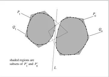
Given a sample S`of points in t−1(`), note that points within their convex hull2ought to receive a “high” value from f`, since the convex hull must be a subset of t−1(`). We need to be able to deal with the case when the convex hull has most or all of S`at its vertices, as would happen for an input distribution D`whose domain is the boundary of a circle, for example. Our general approach is to start out by computing the convex hull P and give maximal value to points inside P. Then give an intermediate value to points in a polygon Q containing P, where Q has fewer edges. We argue that the way Q is chosen ensures that most points in Q are indeed given the correct label.

Theorem 10 Linear separators in the plane are learnable via discriminant functions.

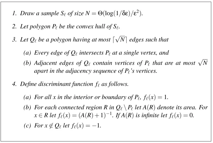
1. Draw a sample S`of size N=Θ(log(1/δε)/ε2).

2. Let polygon P`be the convex hull of S`.

3. Let Q`be a polygon having at mostd√Needges such that

(a) Every edge of Q`intersects P`at a single vertex, and

(b) Adjacent edges of Q` contain vertices of P` that are at most √N

apart in the adjacency sequence of P`’s vertices.

4. Define discriminant function f`as follows.

(a) For all x in the interior or boundary of P`, f`(x) =1.

(b) For each connected region R in Q`\P`let A(R)denote its area. For

x_∈R let f`(x) = (A(R) +1)−1. If A(R)is infinite let f`(x) =0.

(c) For x_6∈Q`let f`(x) =−1.

Figure 5: Assigning values to unlabeled data for linear separators in the plane

Proof Figure 5 shows the algorithm we use to construct discriminant functions; it is not hard to check that the steps can be carried out in polynomial time. Figure 6 illustrates the construction on an example.

Let h : IR2_{−→ {}0,1_}be the hypothesis constructed from f0 and f1. We show below that for `<sub>∈ {</sub>0,1<sub>}</sub>, h−1(`)is a region bounded by O(√N)line segments. We also show that h is consistent with the data, i.e. that for x_∈S`(the unlabeled sample drawn by

A

`), we have h(x) =`. As before, PAC-ness follows from an Occam-algorithm argument; the class of hypotheses has VC dimension

O(√N), sublinear in the sample size.

To show consistency of the hypothesis, suppose x_∈S1, i.e. x is a positive example. Then

f1(x) =1 since x lies in the interior or on the boundary of P1 (rule 4a). By contrast, when f0 is constructed, x lies strictly outside the convex hull of the negative data, so either rule 4b or 4c is applied, giving f0(x)a value less than 1. By symmetry, members of S0are also correctly labeled.

Next we prove our claim that the boundary between the points labeled 0 by h, and the points labeled 1, is indeed simple. (Specifically, h−1(0)and h−1(1)are bounded by O(√N)line segments.) Let L be the line that defines the target linear threshold function t. Let

R

_` be the set of connected regions constructed by

A

<sub>`</sub>that lie between P`and Q`. For R⊆IR2let CH(R)denote the convex hull of R. Observe that

2. at most one element of

R

₀ (respectively,

R

1) may intersect L. (If two of them intersected L, there would be an edge of Q` on the opposite side of L from P`, hence a vertex of P` on the wrong side of L.)

3. for R_∈

R

<sub>`</sub>, CH(R)is a region bounded by three line segments. (R has two “outer” edges and a concave sequence of edges from P`connecting them.)

Suppose that R0∈

R

0intersects R1∈

R

1. Then CH(R0)intersects CH(R1). From Observation 3 above, the boundary of CH(R0) has only 2 line segments on the opposite side of L from P0, and from Observation 1 the boundary of CH(R0)intersects at most 4 elements of

R

1. For all remaining regions R0_1∈

R

₁, either R0_1⊂R0(so that for x∈R10, f1(x)>f0(x)) or R01∩R0= /0(so that again, for

x_∈R0₁, f1(x)> f0(x)).

For `<sub>∈ {</sub>0,1<sub>}</sub>let P<sub>`</sub>0=P`∪ {R` : h(R`) =`}. Note that P`0⊆h−1(`) and has at most 3d

√ N_e

edges.

The portion of t−1(0)not in P₀0_∪P₁0 is divided into O(√N)regions by the remaining edges of

Q0and the two edges of Q1that intersect t−1(0). h is constant within each of these regions, which allows us to deduce that h−1(0)is indeed bounded by a set of line segments of size O(√N). By a similar argument, h−1(1)is bounded by O(√N)lines.

L P

Q

P

Q

1

1

0

0

shaded regions are subsets of andP’ P’

1 0

3.5 Monomials over Attribute Vectors having a Product Distribution.

Recall that a monomial is a boolean function consisting of the conjunction of a set of literals (where a literal is either a boolean attribute or its negation). Despite the simplicity of this class of func-tions, we have not resolved its learnability under the restriction of Definition 1, even for monotone (negation-free) monomials. If

A

₀ and

A

₁ are allowed to be different algorithms (

A

is allowed to treat the positive data differently from the negative data), then the problem does have a simple solu-tion (a property of any class of funcsolu-tions that is learnable from either positive examples only or else negative examples only). f0 from

A

0assigns a value of 1₂ to all boolean vectors.

A

1 uses its data to find a PAC hypothesis, and assigns a value of 1 to examples satisfying that hypothesis, and 0 to other examples.

The following problem arises when

A

is oblivious to whether it is receiving the positive data. The distribution over the negative examples could in fact produce boolean vectors that satisfy some monomial f that differs from target monomial t, but if D(f−1(1)_∩t−1(1))>εthis may give exces-sive error.

In view of the importance of the concept class of monomials, we consider whether they are learnable given that the input distribution D belongs to a given class of probability distributions. This situation is intermediate between knowing D exactly (in which case by Theorem 4 the prob-lem would be solved since monomials are learnable in the presence of uniform misclassification noise (Angluin and Laird, 1988)) and the distribution-independent setting.

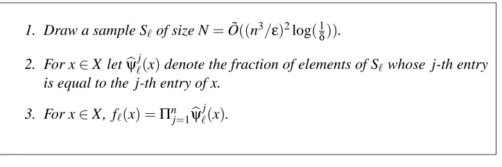
1. Draw a sample S`of size N=O((n˜ 3/ε)2log(1_δ)).

2. For x_∈X letψb`j(x)denote the fraction of elements of S`whose j-th entry

is equal to the j-th entry of x.

3. For x_∈X , f`(x) =Πnj=1ψb

j

`(x).

Figure 7: Algorithm for learning monomials

Theorem 11 Monomials over the boolean domain are learnable via discriminant functions,

pro-vided that the input distribution D is known to be a product distribution.

Comments. We use the algorithm of Figure 7 which simply fits a product distribution to its data and assigns a value to unlabeled vector x that is the estimated likelihood of x. The proof that it works heavily exploits the assumption that D is a product distribution, and does not appear to extend to larger class of distributions (for example, mixtures of product distributions (Cryan et al., 2001; Freund and Mansour, 1999)) or more general classes of boolean functions.

Proof We show that the algorithm given in Figure 7 constructs discriminant functions which, when combined to get h according to Definition 1, ensure that h is PAC.

For x_∼D, x=x1x2. . .xnwhere xjis a 0/1 random variable which is independent of xkfor k6=j.

that value. Let

R

denote the set of relevant attributes and let

I

denote the remaining (irrelevant) attributes.

We say that an example x0=x0₁x0₂. . .x_n0 with t(x0<sub>) =`is ordinary if for all b∈ {0,1} and j∈</sub> {1, . . . ,n<sub>}</sub>such that Prx∼D`(xj=b)>1−

ε

n, we have x0j=b. (Thus, an ordinary example is one that

does not have any “very unusual” attribute values in comparison with random examples having the same label. If there happen to be no bit positions that are very “reliable” for random examples with the same label, then the property becomes vacuous, or true for all bit strings.)

Note that for `<sub>∈ {</sub>0,1<sub>}</sub>, Prx∼D`(x is ordinary)≥1−ε. Consequently, Prx∼D(x is ordinary)≥ 1−ε. We will show that with probability at least 1−δ, all ordinary examples end up correctly labeled.

LetPrbx∈S`(xj=b)denote the empirical probability that xj=b, and we show that sample size N is large enough to ensure that with probability 1₋δ, for b_{∈ {}0,1_}, j_{∈ {}1, . . . ,n_},

|Prbx∈S`(xj=b)−<sub>x</sub>Pr ∼D`

(xj=b)| ≤

ε

8n3. (10)

Applying the same Hoeffding bound as in Theorem 4, it is sufficient that N should satisfy 2e−2N(ε/8n3)2 _≤2nδ2 which is satisfied by N as prescribed in Figure 7.

For `<sub>∈ {</sub>0,1<sub>}</sub>, x<sub>∈</sub>X letψ<sub>`</sub>j(x) denote the probability that a random vector with label`agrees with x on the j-th entry. Note that if t(x) =`thenψb`j(x)(as defined in the algorithm of Figure 7) is an empirical estimate ofψ<sub>`</sub>j(x).

Letψ`(x) =Πjψ<sub>`</sub>j(x). Note that f`(x)is an estimate ofψ`(x)(in the sense that f`(x)converges toψ`(x)as the sample size increases). We know from (10) that

b

ψj

`(x)∈

h

ψj

`(x)−

ε 8n3,ψ

j

`(x) +

ε 8n3

i

.

Ifψ_`j(x)>ε/n, then

b

ψj

`(x)/ψ

j

`(x)∈

h

1₋ 1

8n2,1+ 1 8n2

i

. (11)

Suppose x is ordinary and negative. Observe that f1(x) =0. (This is because x must have an at-tribute value that disagrees with all corresponding atat-tribute values in the positive data.) Furthermore, Equation (11) holds for`=0 and all j, implying that

b

ψ0(x)/ψ0(x)∈

h

1₋ 1

4n,1+ 1 4n

i

. (12)

So with probability 1₋δ, f0(x)>0, since f0(x) =0 would contradict Equation (12) taken with the observation thatψ0(x)>0. Hence with probability 1−δ, all ordinary negative examples are correctly labeled.

Suppose x is ordinary and positive. We will show that with probability 1₋δ, f1(x)/f0(x)>1 for all ordinary positive examples. Observe that for j_∈

R

,ψ₁j(x) =ψb1j(x) =1. (This is because all positive examples must agree on all the relevant attributes.) We have

f1(x) = Πj∈Iψb₁j(x)

For j∈

I

, ψ₁j(x) =ψ₀j(x) (for a product distribution D, the value of an irrelevant attribute is selected independently of the label class of a bit string). Hence Equation (11) applies for`=0 or 1,

j_∈

I

.

f1(x)

f0(x) ≥

(1₋(1/8n2₎₎n

(1+ (1/8n2₎₎n

₁

Πj∈Rψb₀j(x)

.

There exists j∗_∈

R

such that for a fraction at least 1_n of elements x0 _∈S0, x0j∗ 6=xj∗. (Each negative example must disagree with x on at least one relevant attribute.) Hence,

b

ψj∗

0 (x) ≤ 1−(1/n) ψj∗

0 (x) ≤ 1−(1/n) + (ε/8n2)<1−(1/2n). Hence

f1(x)

f0(x) ≥

(1₋(1/8n2₎₎n

(1+ (1/8n2₎₎n

₁

1₋(1/2n)

>1,

as required. Hence with probability 1₋δ, all ordinary positive examples are correctly labeled.

4. Conclusion and Open Problems

The algorithms we have given differ significantly from previous PAC algorithms, which usually work by minimizing the empirical error rate, and arguing that the way a hypothesis is constructed ensures that the true error is close to the empirical error. The constraint that we expressed in Defi-nition 1 forces the positive data and the negative data to be processed independently—an algorithm does not have access to the empirical error.

This lack of access to the empirical error appears to be quite a severe constraint, one that might render certain learning problems intractable in the context of PAC learning. Indeed, we have so far failed to find an algorithm in this setting which learns monomials over the boolean domain, assum-ing no knowledge of the input distribution. We have also not obtained an algorithm for learnassum-ing linear threshold functions in more than two dimensions. Despite those limitations, our positive re-sults have distinguished learnability subject to this constraint from various other constraints on PAC learnability that have been studied in the past.

Clearly, the main open question raised by this paper is to elucidate the relationship between learnability via discriminant functions (Definition 1), and basic PAC learnability. Furthermore, if they are not equivalent, can they be distinguished using a well-known learning problem, such as monomials over the boolean domain?