Journal of Machine Learning Research 18 (2018) 1-50 Submitted 6/17; Published 5/18
Sketched Ridge Regression: Optimization Perspective,
Statistical Perspective, and Model Averaging
Shusen Wang [email protected]
International Computer Science Institute and Department of Statistics University of California at Berkeley
Berkeley, CA 94720, USA
Alex Gittens [email protected]
Computer Science Department Rensselaer Polytechnic Institute Troy, NY 12180, USA
Michael W. Mahoney [email protected]
International Computer Science Institute and Department of Statistics University of California at Berkeley
Berkeley, CA 94720, USA
Editor:Mehryar Mohri
Abstract
We address the statistical and optimization impacts of the classical sketch and Hessian sketch used to approximately solve the Matrix Ridge Regression (MRR) problem. Prior research has quantified the effects of classical sketch on the strictly simpler least squares regression (LSR) problem. We establish that classical sketch has a similar effect upon the optimization properties of MRR as it does on those of LSR: namely, it recovers nearly optimal solutions. By contrast, Hessian sketch does not have this guarantee; instead, the approximation error is governed by a subtle interplay between the “mass” in the responses and the optimal objective value.
For both types of approximation, the regularization in the sketched MRR problem results in significantly different statistical properties from those of the sketched LSR problem. In particular, there is a bias-variance trade-off in sketched MRR that is not present in sketched LSR. We provide upper and lower bounds on the bias and variance of sketched MRR; these bounds show that classical sketch significantly increases the variance, while Hessian sketch significantly increases the bias. Empirically, sketched MRR solutions can have risks that are higher by an order-of-magnitude than those of the optimal MRR solutions.
We establish theoretically and empirically that model averaging greatly decreases the gap between the risks of the true and sketched solutions to the MRR problem. Thus, in parallel or distributed settings, sketching combined with model averaging is a powerful technique that quickly obtains near-optimal solutions to the MRR problem while greatly mitigating the increased statistical risk incurred by sketching.
Keywords: Randomized Linear Algebra, Matrix Sketching, Ridge Regression
c
Wang, Gittens, and Mahoney
1. Introduction
Regression is one of the most fundamental problems in machine learning. The simplest and most thoroughly studied regression model is least squares regression (LSR). Given features X= [xT
1;. . . ,xTn]∈Rn×d and responses y = [y1, . . . , yn]T ∈Rn, the LSR problem
minwkXw−yk22can be solved inO(nd2) time using the QR decomposition or inO(ndt) time
using accelerated gradient descent algorithms. Here, t is the number of iterations, which depends on the initialization, the condition number ofXTX, and the stopping criterion.
This paper considers thendproblem, where there is much redundancy inX. Matrix sketching, as used in the paradigm of Randomized Linear Algebra (RLA) (Mahoney, 2011; Woodruff, 2014; Drineas and Mahoney, 2016), aims to reduce the size of X while limiting information loss; the sketching operation can consist of sampling a subset of the rows ofX, or forming linear combinations of the rows ofX. Either operation is modeled mathematically by multiplication with a sketching matrixS to form the sketchSTX. The sketching matrix S ∈Rn×s satisfies d < s n so that STX generically has the same rank but much fewer
rows asX. Sketching has been used to speed up LSR (Drineas et al., 2006b, 2011; Clarkson and Woodruff, 2013; Meng and Mahoney, 2013; Nelson and Nguyˆen, 2013) by solving the sketched LSR problem minwkSTXw−STyk22 instead of the original LSR problem. Solving sketched LSR costs either O(sd2 +T
s) time using the QR decomposition or O(sdt+Ts)
time using accelerated gradient descent algorithms, where t is as defined previously1 and
Ts is the time cost of sketching. For example, Ts =O(ndlogs) whenS is the subsampled
randomized Hadamard transform (Drineas et al., 2011), and Ts = O(nd) when S is a
CountSketch matrix (Clarkson and Woodruff, 2013).
There has been much work in RLA on analyzing the quality of sketched LSR with different sketching methods and different objectives; see the reviews (Mahoney, 2011; Woodruff, 2014; Drineas and Mahoney, 2016) and the references therein. The concept of sketched LSR originated in the theoretical computer science literature, e.g., Drineas et al. (2006b, 2011), where the behavior of sketched LSR was first studied from an optimization perspective. Let w? be the optimal LSR solution and ˜w be the solution to sketched LSR.
This line of work established that ifs=O(d/+poly(d)), then the objective valuekXw˜−y 2 2
is at most (1+) times greater than kXw? −y 2
2. These works also bounded kw˜ −w ?k2
2
in terms of the difference in the objective function values at ˜w and w? and the condition
number ofXTX.
A more recent line of work has studied sketched LSR from a statistical perspective: Ma et al. (2015); Raskutti and Mahoney (2016); Pilanci and Wainwright (2015); Wang et al. (2017c) considered statistical properties of sketched LSR such as the bias and variance. In particular, Pilanci and Wainwright (2015) showed that the solutions to sketched LSR have much higher variance than the optimal solutions.
Both of these perspectives are important and of practical interest. The optimization perspective is relevant when the approximate solution is used to initialize an (expensive) iterative optimization algorithm; the statistical perspective is relevant in machine learning and statistics applications where the approximate solution is directly used in lieu of the optimal solution.
Sketched Ridge Regression
In practice, regularized regression, e.g., ridge regression and LASSO, exhibit more attractive bias-variance trade-offs and generalization errors than vanilla LSR. Furthermore, the matrix generalization of LSR, where multiple responses are to be predicted, is often more useful than LSR. However, the properties of sketched regularized matrix regression are largely unknown. Hence, we consider the question: how does our understanding of the optimization and statistical properties of sketched LSR generalize to sketched regularized regression problems? We answer this question for the sketched matrix ridge regression (MRR) problem.
Recall thatX isn×d. LetY∈Rn×m denote a matrix of corresponding responses. We
study the MRR problem
min W
n
f(W) , n1XW−Y 2
F +γkWk 2 F
o
, (1)
which has optimal solution
W? = (XTX+nγId)†XTY. (2)
Here, (·)† denotes the Moore-Penrose inversion operation. LSR is a special case of MRR, with m= 1 and γ = 0. The optimal solution W? can be obtained in O(nd2+nmd) time
using a QR decomposition ofX. Sketching can be applied to MRR in two ways:
Wc = (XTSSTX+nγId)†(XTSSTY), (3) Wh = (XTSSTX+nγId)†XTY. (4)
Following the convention of Pilanci and Wainwright (2015); Wang et al. (2017a), we call
Wctheclassical sketchandWh theHessian sketch. Table 1 lists the time costs of the three solutions to MRR.
Table 1: The time cost of the solutions to MRR. Here Ts(X) and Ts(Y) denote the time
cost of forming the sketchesSTX∈
Rs×d and STY ∈Rs×m.
Solution Definition Time Complexity
Optimal Solution (2) O(nd2+nmd)
Classical Sketch (3) O(sd2+smd) +T
s(X) +Ts(Y)
Hessian Sketch (4) O(sd2+nmd) +T
s(X)
1.1 Main Results and Contributions
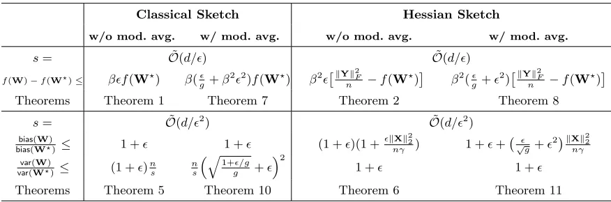
We summarize all of our upper bounds in Table 2. Our optimization analysis bounds the gap between the objective function values at the sketched and optimal solutions, while our statistical analysis quantifies the behavior of the bias and variance of the sketched solutions relative to those of the true solutions.
Wang, Gittens, and Mahoney
Table 2: A summary of our main results. In the table,Wis the solution of classical/Hessian sketch with or without model averaging (mod. avg.); W? is the optimal solution;
g is the number of models used in model averaging; andβ = kXk22
kXk2 2+nγ
≤1, where
γ is the regularization parameter. For conciseness, we take the sketching matrix
S∈Rn×sto correspond to Gaussian projection, SRHT, or shrinkage leverage score
sampling. Similar but more complex expressions hold for uniform sampling (with or without model averaging) and CountSketch (only without model averaging.) All the bounds hold with constant probability. The notation ˜O conceals logarithmic factors.
Classical Sketch Hessian Sketch
w/o mod. avg. w/ mod. avg. w/o mod. avg. w/ mod. avg.
s= O˜(d/) O˜(d/)
f(W)−f(W?)≤ βf(W?) β( g+β
22)f(
W?) β2kYk2
F
n −f(W ?)
β2( g +
2)kYk2
F
n −f(W ?)
Theorems Theorem 1 Theorem 7 Theorem 2 Theorem 8
s= O˜(d/2) O˜(d/2)
bias(W)
bias(W?) ≤ 1 + 1 + (1 +)(1 +
kXk2 2
nγ ) 1 ++
√
g +
2kXk2 2 nγ var(W)
var(W?) ≤ (1 +)
n s
n s
q
1+/g
g +
2
1 + 1 +
Theorems Theorem 5 Theorem 10 Theorem 6 Theorem 11
• Classical sketch achieves relative error in the objective value. With sketch size s = ˜
O(d/), the sketched solution satisfies f(Wc)≤(1 +)f(W?).
• Hessian sketch does not achieve relative error in the objective value. In particular, if
1
nkYk2F is much larger than f(W?), then f(Wh) can be far larger than f(W?).
• For both classical and Hessian sketch, the relative quality of approximation often improves as the regularization parameterγ increases (becauseβ decreases).
We then study classical and Hessian sketch from the statistical perspective, by modelingY=XW0+Ξas the sum of a true linear model and random noise, decomposing
the risk R(W) = EkXW−XW0k2F into bias and variance terms, and bounding these
terms. We draw the following conclusions (see Theorems 4, 5, 6 for the details):
• The bias of classical sketch can be nearly as small as that of the optimal solution. The variance is Θ n
s
times that of the optimal solution; this bound is optimal. Therefore over-regularization2 should be used to supress the variance. (Asγ increases, the bias increases, and the variance decreases.)
Sketched Ridge Regression
• Since Hessian sketch uses the whole of Y, the variance of Hessian sketch can be close to that of the optimal solution. However, Hessian sketch incurs a high bias, especially whennγ is small compared tokXk22. This indicates that over-regularization is necessary for Hessian sketch to deliver solutions with low bias.
Our empirical evaluations bear out these theoretical results. In particular, in Section 4, we show in Figure 3 that even when the regularization parameterγ is fine-tuned, the risks of classical and Hessian sketch are worse than that of the optimal solution by an order of magnitude. This is an empirical demonstration of the fact that the near-optimal properties of sketch from the optimization perspective are much less relevant in a statistical setting than its sub-optimal statistical properties.
We propose to use model averaging, which averages the solutions ofgsketched MRR problems, to attain lower optimization and statistical errors. Without ambiguity, we denote model-averaged classical and Hessian sketches by Wc and Wh, respectively. Theorems 7, 8, 10, 11 establish the following results:
• Classical Sketch. Model averaging decreases the objective function value and the variance and does not increase the bias. Specifically, with the same sketch size s, model averaging ensures f(Wfc()W−f?()W?) and
var(Wc)
var(W?) respectively decrease to almost 1g of those of classical sketch without model averaging, provided thatsd. See Table 2 for the details.
• Hessian Sketch. Model averaging decreases the objective function value and the bias and does not increase the variance.
In the distributed setting, the feature-response pairs (x1,y1),· · ·,(xn,yn) ∈Rd×Rm are
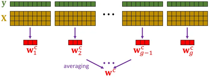
divided among g machines. Assuming that the data have been shuffled randomly, each machine contains a sketch of the MRR constructed by uniformly sampling rows from the data set without replacement. We illustrate this procedure in Figure 1. In this setting, the model averaging procedure communicates the g local models only once to return the final estimate; this process has very low communication and latency costs, and suggests two further applications of classical sketch with model averaging:
• Model Averaging for Machine Learning. When a low-precision solution is acceptable, model averaging can be used in lieu of distributed numerical optimization algorithms requiring multiple rounds of communication. If ng is large enough compared to d
and the row coherence of X is small, then “one-shot” model averaging has bias and variance comparable to the optimal solution.
• Model Averaging for Optimization. If a high-precision solution to MRR is required, then an iterative numerical optimization algorithm must be used. The cost of such algorithms heavily depends on the quality of the initialization.3 A good initialization reduces the number of iterations needed to reach convergence. The averaged model
3. For example, the conjugate gradient method satisfies kW(t)−W?k2F kW(0)−W?k2
F
≤θt
1and stochastic block coordinate
descent (Tu et al., 2016) satisfies Ef(W(t))−f(W?)
f(W(0))−f(W?) ≤θ
t
2. Here W(t) is the output of the t-th iteration;
Wang, Gittens, and Mahoney
⋯
"
#
$
%&$
'&
$
()%&$
(&$
&⋯
averaging
Figure 1: Using model averaging with the classical sketch in the distributed setting to approximately solve LSR.
is provably close to the optimal solution, so model averaging provides a high-quality initialization for more expensive algorithms.
1.2 Prior Work
The body of work on sketched LSR mentioned earlier (Drineas et al., 2006b, 2011; Clarkson and Woodruff, 2013; Meng and Mahoney, 2013; Nelson and Nguyˆen, 2013) shares many similarities with our results. However, the theories of sketched LSR developed from the optimization perspective do not obviously extend to MRR, and the statistical analysis of LSR and MRR differ: among other differences, LSR is unbiased while MRR is biased and therefore has a bias-variance tradeoff that must be considered.
Lu et al. (2013) has considered a different application of sketching to ridge regression: they assume d n, reduce the number of features in X using sketching, and conduct statistical analysis. Our setting differs in that we consider n d, reduce the number of samples by sketching, and allow for multiple responses.
The model averaging analyzed in this paper is similar in spirit to the AvgMalgorithm
of (Zhang et al., 2013). When classical sketch is used with uniform row sampling without replacement, our model averaging procedure is a special case of AvgM. However, our results
do not follow from those of (Zhang et al., 2013). First, we make no assumption on the data, X and Y, and the model (parameters), W. Second, we study both the optimization objective,kXWc−XW?k2
F, and the statistical objective,EkXWc−XW0k2F, whereWcis
the average of the approximate solutions obtained used classical sketch,W0 is the unknown
ground truth, andW?is the optimal solution based on the observed data; they studied solely
Sketched Ridge Regression
Iterative Hessian sketch has been studied in Pilanci and Wainwright (2015); Wang et al. (2017a,b). By way of comparison, all the algorithms in this paper are “one-shot” rather than iterative. This work has connections to the contemporary works (Avron et al., 2017; Thanei et al., 2017; Derezinski and Warmuth, 2017, 2018). Avron et al. (2017) studied classical sketch from the optimization perspective; Thanei et al. (2017) studied LSR with model averaging; Derezinski and Warmuth (2017, 2018) studied linear regression with volume sampling for experimental design.
1.3 Paper Organization
Section 2 defines our notation and introduces the sketching schemes we consider. Section 3 presents our theoretical results. Sections 4 and 5 conduct experiments to verify our theories and demonstrates the efficacy of model averaging. Section 6 sketches the proofs of our main results. Complete proofs are provided in the appendix.
2. Preliminaries
Throughout, we take In to be the n×n identity matrix and0 to be a vector or matrix of
all zeroes of the appropriate size. Given a matrixA= [aij], the i-th row is denoted by ai:,
and thej-th column is denoted bya:j. The Frobenius and spectral norms ofAare written
as, respectively,kAkF and kAk2. The set {1,2,· · ·, n} is written [n]. LetO, Ω, and Θ be the standard asymptotic notation, and let ˜O conceal logarithmic factors.
Throughout, we fix X∈Rn×d as our matrix of features. We setρ= rank(X) and write
the SVD of X as X = UΣVT, where U, Σ, V are respectively n×ρ, ρ×ρ, and d×ρ
matrices. We letσ1≥ · · · ≥σρ>0 be the singular values ofX. The Moore-Penrose inverse
ofX is defined byX†=VΣ−1UT. The row leverage scores ofX arel
i=ku:ik22 fori∈[n].
The row coherence of X is µ(X) = nρmaxiku:ik22. Throughout, we let µ be shorthand for µ(X). The notation defined in Table 3 is used throughout this paper.
Matrix sketching attempts to reduce the size of large matrices while minimizing the loss of spectral information that is useful in tasks like linear regression. We denote the process of sketching a matrixX∈Rn×dbyX0=STX. Here, S∈Rn×sis called a sketching matrix
and X0 ∈Rs×d is called a sketch of X. In practice, except for Gaussian projection (where
the entries of S are i.i.d. sampled from N(0,1/s)), the sketching matrix S is not formed explicitly.
Matrix sketching can be accomplished by random sampling or random projection.
Random samplingcorresponds to sampling rows ofXi.i.d. with replacement according to given row sampling probabilitiesp1,· · ·, pm∈(0,1). The corresponding (random) sketching
matrixS ∈Rn×s has exactly one non-zero entry, whose position indicates the index of the
selected row in each column; in practice, thisSis not explicitly formed. Uniform sampling
fixes p1 = · · · = pn = n1. Leverage score sampling sets pi proportional to the (exact
Wang, Gittens, and Mahoney
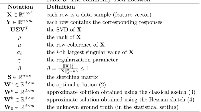
Table 3: The commonly used notation. Notation Definition
X∈Rn×d each row is a data sample (feature vector)
Y∈Rn×m each row contains the corresponding responses
UΣVT the SVD ofX
ρ the rank ofX
µ the row coherence ofX
σi thei-th largest singular value ofX γ the regularization parameter
β β= kXk22
kXk2 2+nγ
≤1 S∈Rn×s the sketching matrix
W?∈
Rd×m the optimal solution (2)
Wc∈
Rd×m approximate solution obtained using the classical sketch (3)
Wh∈
Rd×m approximate solution obtained using the Hessian sketch (4)
W0∈Rd×m the unknown ground truth (in the statistical setting)
2015). The sampling probabilities of shrinked leverage score sampling are defined by
pi = 12 Pnli j=1lj +
1 n
.4
The exact leverage scores are unnecessary in practice; constant-factor approximation to the leverage scores is sufficient. Leverage scores can be efficiently approximated by the algorithms of (Drineas et al., 2012). Let l1,· · · , ln be the true leverage scores. We denote
the approximate leverages byel1,· · · ,eln and require that they satisfy
˜
lq∈[lq, τ lq] for all q∈[n], (5)
where τ ≥ 1 indicates the quality of approximation. We then use pq = ˜lq/Pj˜lj as
the sampling probabilities. One can obtain the same accuracies when using approximate leverage scores in place of the true leverage scores by increasing s by a factor of τ, so as long asτ is a small constant, the orders of the sketch sizes when using exact or approximate leverage score sampling are the same. Thus we do not distinguish between exact and approximate leverage scores in this paper. For shrinked leverage score sampling, we define the sampling probabilities
pi = 12
˜ li Pn
j=1˜lj +
1 n
for i= 1, . . . , n. (6)
Gaussian projection is also well-known as the prototypical Johnson-Lindenstrauss transform (Johnson and Lindenstrauss, 1984). Let G ∈ Rn×s be a standard Gaussian
matrix, i.e., each entry is sampled independently from N(0,1). The matrix S= √1
sG is a
Gaussian projection matrix. It takes O(nds) time to apply S ∈ Rn×s to any n×d dense
matrix, which makes Gaussian projection computationally inefficient relative to other forms of sketching.
4. In fact,pi can be any convex combination of li
Pn
j=1lj and
1
n (Ma et al., 2015). We use the weight
1 2 for
Sketched Ridge Regression
The Subsampled randomized Hadamard transform (SRHT) (Drineas et al., 2011; Lu et al., 2013; Tropp, 2011) is a more efficient alternative to Gaussian projection. Let Hn ∈Rn×n be the Walsh-Hadamard matrix with +1 and −1 entries, D ∈Rn×n be a
diagonal matrix with diagonal entries sampled uniformly from{+1,−1}, and P∈Rn×s be
the uniform row sampling matrix defined above. The matrix S = √1nDHnP∈Rn×s is an
SRHT matrix, and can be applied to any n×d matrix in O(ndlogs) time. In practice, the subsampled randomized Fourier transform (SRFT) (Woolfe et al., 2008) is often used in lieu of the SRHT, because the SRFT exists for all values of n, whereas Hn exists only
for some values ofn. Their performance and theoretical analyses are very similar.
CountSketch can be applied to any X ∈ Rn×d inO(nd) time (Charikar et al., 2004;
Clarkson and Woodruff, 2013; Meng and Mahoney, 2013; Nelson and Nguyˆen, 2013; Pham and Pagh, 2013; Weinberger et al., 2009). Though more efficient to apply, CountSketch requires a larger sketch size than Gaussian projections, SRHT, and leverage score sampling to attain the same theoretical guarantees. Interested readers can refer to (Woodruff, 2014) for a detailed description of CountSketch. Unlike the other sketching methods mentioned here, model averaging with CountSketch may not be theoretically sound. See Remark 5 for further discussion.
3. Main Results
Sections 3.1 and 3.2 analyze sketched MRR from, respectively, the optimization and statistical perspectives. Sections 3.3 and 3.4 capture the impacts of model averaging on, respectively, the optimization and statistical properties of sketched MRR.
We described six sketching methods in Section 2. For simplicity, in this section, we refer to leverage score sampling, shrinked leverage score sampling, Gaussian projection, and SRHT as the four sketching methods while we refer to uniform sampling and CountSketch by name. Throughout, letµbe the row coherence ofXandβ = kXk22
kXk2 2+nγ
≤1.
3.1 Sketched MRR: Optimization Perspective
Theorem 1 shows thatf(Wc), the objective value of classical sketch, is close to the optimal objective valuef(W?), and that the approximation quality improves as the regularization
parameterγ increases.
Theorem 1 (Classical Sketch) Let β = kXk22
kXk2 2+nγ
≤ 1. For the four sketching methods
with s= ˜O d
, uniform sampling with s= O µdlog d
, and CountSketch with s=O d2
, the inequality
f(Wc)−f(W?) ≤ β f(W?)
holds with probability at least 0.9. The uncertainty is with respect to the random choice of sketching matrix.
Wang, Gittens, and Mahoney
of the columns ofX—andγ is small, thenf(W?) is close to zero, and consequently f(W?)
can be far smaller than 1nkYk2F. Therefore, in this case which is ideal for MRR, f(Wh) is not close tof(W?) and our theory suggests Hessian sketch does not perform as well as
classical sketch. This is verified by our experiments (see Figure 2), which show that unless
γ is large or a large portion ofY is outside the column space ofX, the ratio ff((WW?h)) can be large.
Theorem 2 (Hessian Sketch) Let β = kXk22
kXk2 2+nγ
≤ 1. For the four sketching methods
with s = ˜O d
, uniform sampling with s =O µdlog d
, and CountSketch with s =O(d2), the inequality
f(Wh)−f(W?) ≤ β2kYk2
F
n −f(W
?).
holds with probability at least 0.9. The uncertainty is with respect to the random choice of sketching matrix.
These two results imply that f(Wc) and f(Wh) can be close to f(W?). When this is
the case, curvature of the objective function ensures that the sketched solutions Wc and
Wh are close to the optimal solution W?. Lemma 3 bounds the Mahalanobis distance
kM(W−W?)k2
F. Here Mis any non-singular matrix; in particular, it can be the identity
matrix or (XTX)1/2. Lemma 3 is a consequence of Lemma 25.
Lemma 3 (Mahalanobis Distance) Let f be the objective function of MRR defined in (1), W ∈ Rd×m be arbitrary, and W? be the optimal solution defined in (2). For any
non-singular matrix M, the Mahalanobis distance satisfies 1
n
M(W−W?)
2
F ≤
f(W)−f(W?) σ2
min
(XTSSTX+nγI
d)1/2M−1
.
By choosingM= (XTX)1/2, we can bound 1
nkXW−XW ?k2
F in terms of the difference
in the objective values:
1 n
XW−XW?
2
F ≤ β
f(W)−f(W?)
,
whereβ = kXk22
kXk2 2+nγ
≤1. With Lemma 3, we can directly apply Theorems 1 or 2 to bound
1
nkXWc−XW?k2F or n1kXWh−XW?k2F. 3.2 Sketched MRR: Statistical Perspective
We consider the following fixed design model. LetX∈Rn×dbe the observed feature matrix, W0 ∈Rd×m be the true and unknown model, Ξ∈Rn×m contain unknown random noise,
and
Y = XW0+Ξ (7)
be the observed responses. We make the following standard weak assumptions on the noise:
Sketched Ridge Regression
We observe Xand Y and seek to estimate W0.
We can evaluate the quality of the estimate by the risk:
R(W) = 1nEXW−XW0 2
F, (8)
where the expectation is taken w.r.t. the noise Ξ. We study the risk functions R(W?),
R(Wc), andR(Wh) in the following.
Theorem 4 (Bias-Variance Decomposition) We consider the data model described in this subsection. LetW beW?,Wc, or Wh, as defined in (2),(3), or (4), respectively; then
the risk function can be decomposed as
R(W) = bias2(W) +var(W).
Recall the SVD of X defined in Section 2: X=UΣVT. The bias and variance terms can
be written as
bias W?
= γ√n (Σ
2+nγI
ρ)−1ΣVTW0
F,
var W?
= ξn2
Iρ+nγΣ
−2−1
2
F,
bias Wc
= γ√n
U
TSSTU+nγΣ−2†
Σ−1VTW 0
F,
var Wc
= ξn2
U
TSSTU+nγΣ−2†
UTSST
2
F,
bias Wh
= γ√n
Σ−2+UTSSTU−Iρ
nγ
UTSSTU+nγΣ−2†
ΣVTW 0
F,
var Wh
= ξ2 n
U
TSSTU+nγΣ−2†
2
F.
The functions bias(W?) and var(W?) are deterministic. The randomness inbias(Wc),
var(Wc), bias(Wh), andvar(Wh) all arises from the sketching matrix S.
Throughout this paper, we compare the bias and variance of classical sketch and Hessian sketch to those of the optimal solution W?. We first study the bias, variance, and risk of W?, which will help us understand the subsequent comparisons. We can assume that Σ2 =VTXTXV is linear in n; this is reasonable because XTX=Pn
i=1xixTi and V is an
orthogonal matrix.
• Bias. The bias of W? is independent of nand is increasing with γ. The bias is the
price paid for using regularization to decrease the variance; for least squares regression,
γ is zero, and the bias is zero.
• Variance. The variance of W? is inversely proportional to n. As n grows, the
variance decreases to zero, and we must also decreaseγ to ensure that the sum of the squared bias and variance decreases to zero.
• Risk. Note that W? is not the minimizer of R(·); W
0 is the minimizer because R(W0) = 0. Nevertheless, because W0 is unknown, W? for a carefully chosen γ is
Wang, Gittens, and Mahoney
Theorem 5 provides upper and lower bounds on the bias and variance of solutions obtained using classical sketch. In particular, we see that that bias(Wc) is within a factor of (1±) of bias(W?). However, var(Wc) can be Θ(n
s) times worse than var(W
?). The
absolute value of var(Wc) is inversely proportional to s, whereas the absolute value of
bias(Wc) is almost independent ofs.
Theorem 5 (Classical Sketch) Assume s ≤ n. For Gaussian projection and SRHT sketching with s = ˜O(d
2), uniform sampling with s = O(
µdlogd
2 ), or CountSketch with
s=O(d2
2), the inequalities
1− ≤ biasbias((WW?c)) ≤ 1 +, (1−)n
s ≤
var(Wc)
var(W?) ≤ (1 +)ns
hold with probability at least 0.9. For shrinked leverage score sampling with s=O(dlog2 d),
these inequalities, except for the lower bound on the variance, hold with probability at least 0.9. Here the randomness comes from the sketching matrix S.
Remark 1 To establish an upper (lower) bound on the variance, we need an upper (lower) bound on kSk2
2. There is no nontrivial upper nor lower bound on kSk22 for leverage score
sampling, so the variance of leverage score sampling cannot be bounded. Shrinked leverage score sampling satisfies the upper bound kSk22 ≤ 2sn; but kSk22 does not have a nontrivial lower bound, so there is no nontrivial lower bound on the variance of shrinked leverage score. Remark 4 explains the nonexistence of the relevant bounds on kSk2
2 for both variants
of leverage score sampling.
Theorem 6 establishes similar upper and lower bounds on the bias and variance of solutions obtained using Hessian sketch. The situation is the reverse of that with classical sketch: the variance of Wh is close to that of W? if s is large enough, but as the
regularization parameter γ goes to zero, bias(Wh) becomes much larger than bias(W?).
The theory suggest that Hessian sketch should be preferred over classical sketch whenY is very noisy, because Hessian sketch does not magnify the variance.
Theorem 6 (Hessian Sketch) For the four sketching methods with s= ˜O(d
2), uniform
sampling with s=O(µdlog2 d), and CountSketch with s=O(d 2
2), the inequalities
bias(Wh)
bias(W?) ≤ (1 +) 1 +
kXk2 2
nγ
,
1− ≤ varvar((WW?h)) ≤ 1 +
hold with probability at least 0.9. Further assume that the ρ-th singular value of Xsatisfies
σ2
ρ ≥ nγ , then
bias(Wh)
bias(W?) ≥ 1+1
σ2
ρ
nγ −1
Sketched Ridge Regression
The lower bound on the bias shows that the solution from Hessian sketch can exhibit a much higher bias than the optimal solution. The gap between bias(Wh) and bias(W?)
can be lessened by increasing the regularization parameterγ, but such over-regularization increases the baseline bias(W?) itself. It is also worth mentioning that unlike bias(W?)
andbias(Wc),bias(Wh) is not monotonically increasing withγ, as is empirically verified in Figure 3.
In sum, our theory shows that the classical and Hessian sketches are not statistically comparable to the optimal solutions: classical sketch has too high a variance, and Hessian sketch has too high a bias for reasonable amounts of regularization. In practice, the regularization parameter γ should be tuned to optimize the prediction accuracy. Our experiments in Figure 3 show that even with carefully chosen γ, the risks of classical and Hessian sketch can be higher than the risk of the optimal solution by an order of magnitude. Formally speaking, minγR(Wc) minγR(W?) and minγR(Wh) minγR(W?) hold in
practice.
Our empirical study in Figure 3 suggests classical and Hessian sketch both require over-regularization, i.e., setting γ larger than is best for the optimal solution W?. Formally
speaking, argminγR(Wc) > argminγR(W?) and argmin
γR(Wh) > argminγR(W?).
Although this is the case for both types of sketching, the underlying explanations are different. Classical sketches have a high variance, so a large γ is required to supress their variance (the variance is non-increasing withγ). Hessian sketches magnify the bias when γ
is small, so a reasonably largeγ is necessary to lower their bias.
3.3 Model Averaging: Optimization Perspective
We consider model averaging as a method to increase the accuracy of sketched MRR solutions. The model averaging procedure is straightforward: one independently draws
g sketching matrices S1,· · ·,Sg ∈ Rn×s, uses these to form g sketched MRR solutions,
denoted by{Wci}gi=1 or{Wih}gi=1, and averages these solutions to obtain the final estimate
Wc = g1Pg
i=1Wic or Wh = 1g Pg
i=1Whi. Practical applications of model averaging are
enumerated in Section 1.1.
Theorems 7 and 8 present guarantees on the optimization accuracy of using model averaging on classical/Hessian sketch solutions. We can contrast these with the guarantees provided for sketched MRR in Theorems 1 and 2. For classical sketch with model averaging, we see that when≤ 1g, the bound onf(Wh)−f(W?) is proportional to/g. From Lemma 3
we see that the distance betweenWc andW? also decreases accordingly. Theorem 7 (Classical Sketch with Model Averaging) Let β = kXk22
kXk2 2+nγ
≤ 1. For
the four methods, let s = ˜O d
, and for uniform sampling, let s = O µdlog d
, then the inequality
f(Wc)−f(W?) ≤ β g +β
2
2f(W?)
holds with probability at least 0.8. Here the randomness comes from the choice of sketching matrices.
For Hessian sketch with model averaging, if < g1, then the bound onf(Wh)−f(W?)
Wang, Gittens, and Mahoney
Theorem 8 (Hessian Sketch with Model Averaging) Let β = kXk22
kXk2 2+nγ
≤1. For the
four methods lets= ˜O d
, and for uniform sampling lets=O µdlog d
, then the inequality
f(Wh)−f(W?) ≤ β2 g +
2 kYk2F
n −f(W ?)
holds with probability at least 0.8. Here the randomness comes from the choice of sketching matrices.
3.4 Model Averaging: Statistical Perspective
Model averaging has the salutatory property of reducing the risks of the classical and Hessian sketches. Our first result conducts a bias-variance decomposition for the averaged solution of the sketched MRR problem.
Theorem 9 (Bias-Variance Decomposition) We consider the fixed design model (7). Decompose the risk function defined in (8)as
R(W) = bias2(W) +var(W).
The bias and variance terms are
bias Wc
= γ√n
1 g g X i=1 UTS
iSTi U+nγΣ −2†
Σ−1VTW 0 F ,
var Wc
= ξ 2 n 1 g g X i=1 UTS
iSTiU+nγΣ −2†
UTS iSTi
2 F ,
bias Wh
= γ√n
1 g g X i=1
Σ−2+UTSiSTiU−Iρ
nγ
UTS
iSTiU+nγΣ −2†
ΣVTW 0 F ,
var Wh
= ξ 2 n 1 g g X i=1 UTS
iSTiU+nγΣ −2†
2 F .
Theorems 10 and 11 provide upper bounds on the bias and variance of averaged sketched MRR solutions for, respectively, classical sketch and Hessian sketch. We can contrast them with Theorems 5 and 6 to see the statistical benefits of model averaging. Theorem 10 shows that when g ≈ n
s, classical sketch with model averaging yields a solution with comparable
bias and variance to the optimal solution.
Theorem 10 (Classical Sketch with Model Averaging) For the four sketching meth-ods with s= ˜O d2
, or uniform sampling with s=O µdlog2 d
, the inequalities
bias(Wc)
bias(W?) ≤ 1 + and
var(Wc) var(W?) ≤
n s
√1 +
√
h +
2
,
where h = min{g, Θ(n
s)}, hold with probability at least 0.8. The randomness comes from
the choice of sketching matrices.
Theorem 11 shows that model averaging decreases the bias of Hessian sketch without increasing the variance. For Hessian sketch without model averaging, recall thatbias(Wh) is
larger thanbias(W?) by a factor ofO(kXk2
2/(nγ)). Theorem 11 shows that model averaging
Sketched Ridge Regression
Theorem 11 (Hessian Sketch with Model Averaging) For the four sketching meth-ods with s= ˜O d2
, or uniform sampling with s=O µdlog2 d
, the inequalities
bias(Wh)
bias(W?) ≤ 1 ++
√ g +
2kXk22
nγ and
var(Wh)
var(W?) ≤ 1 +
hold with probability at least 0.8. Here the randomness comes from the choice of sketching matrices.
4. Experiments on Synthetic Data
We conduct experiments on synthetic data to verify our theory. Section 4.1 describes the data model and experiment settings. Sections 4.2 and 4.3 empirically study classical and Hessian sketch from the optimization and statistical perspectives, respectively, to verify Theorems 1, 2, 5, and 6. Sections 4.4 and 4.5 study model averaging from the optimization and statistical perspectives, respectively, to corroborate Theorems 7, 8, 10, and 11.
4.1 Settings
Following (Ma et al., 2015; Yang et al., 2016), we constructX=Udiag(σ)VT ∈
Rn×d and y=Xw0+ε∈Rn in the following way.
• We take U be the matrix of left singular vectors of A ∈Rn×d which is constructed
in the following way. (Note that A and X are different.) Let the rows of A be i.i.d. sampled from a multivariatet-distribution with covariance matrixCandv= 2 degree of freedom, where the (i, j)-th entry of C ∈Rd×d is 2×0.5|i−j|. Constructing A in
this manner ensures that it has high row coherence.
• Let the entries of b∈Rd be equally spaced between 0 and−6 and takeσi= 10bi for
all i∈[d].
• Let V ∈ Rd×d be an orthonormal basis for the column range of a d×d standard
Gaussian matrix.
• Letw0= [10.2d; 0.110.6d;10.2d].
• Take the entries of ε∈Rn to be i.i.d. samples from the N(0, ξ2) distribution.
This construction ensures that X has high row coherence, and its condition number is
κ(XTX) = 1012. LetS∈
Rn×sbe any of the six sketching methods considered in this paper.
We fix n= 105,d= 500, ands= 5,000. Since the sketching methods are randomized, we
repeat each trial 10 times with idependent sketches and report averaged results.
4.2 Sketched MRR: Optimization Perspective
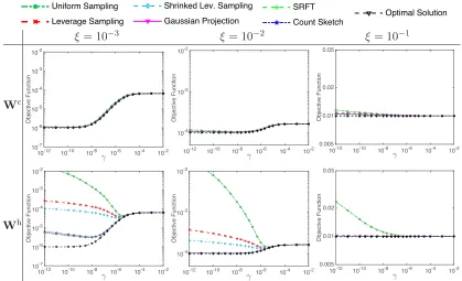
We seek to empirically verify Theorems 1 and 2 which study classical and Hessian sketches, respective, from the optimization perspective. In Figure 2, we plot the objective function value f(w) = n1kXw−yk2
2+γkwk22 againstγ, under different settings ofξ (the standard
Wang, Gittens, and Mahoney
g
050
Variance
10-6 10-5 10-4
Uniform Sampling Leverage Sampling Shrinked Lev. Sampling Gaussian Projection SRFT
Count Sketch Optimal Solution
g
050
Variance
10-6 10-5
10-4
Uniform Sampling
Leverage Sampling
Shrinked Lev. Sampling
Gaussian Projection
SRFT
Count Sketch
Optimal Solution
g 050
Variance
10-6 10-5 10-4
Uniform Sampling
Leverage Sampling
Shrinked Lev. Sampling
Gaussian Projection
SRFT
Count Sketch
Optimal Solution
g 050
Variance
10-6 10-5 10-4
Uniform Sampling
Leverage Sampling
Shrinked Lev. Sampling
Gaussian Projection
SRFT
Count Sketch
Optimal Solution
Figure 20: .
.
ξ= 10−3 ξ= 10−2 ξ= 10−1
Wc
γ
10-12 10-10 10-8 10-6 10-4 10-2
Objective Function
10-7 10-6 10-5 10-4 10-3 10-2
γ
10-12 10-10 10-8 10-6 10-4 10-2
Objective Function
10-4 10-3 10-2
γ
10-12 10-10 10-8 10-6 10-4 10-2
Objective Function
0.005 0.01 0.02 0.05
Wh
γ
10-12 10-10 10-8 10-6 10-4 10-2
Objective Function
10-7 10-6 10-5 10-4 10-3 10-2
γ
10-12 10-10 10-8 10-6 10-4 10-2
Objective Function
10-4 10-3 10-2
γ
10-12 10-10 10-8 10-6 10-4 10-2
Objective Function
0.005 0.01 0.02 0.05
Figure 2: An empirical study of classical and Hessian sketch from the optimization perspective. Thex-axis is the regularization parameter γ (log scale); the y-axis is the objective function values (log scale). Here ξ is the standard deviation of the Gaussian noise added to the response.
sketching methods. The results verify our theory: the objective value of the solution from the classical sketch, wc, is always close to optimal; and the objective value of the solution from the Hessian sketch,wh, is much worse than the optimal value when γ is small and y
is mostly in the column space of X.
4.3 Sketched MRR: Statistical Perspective
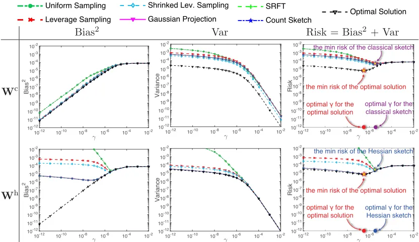
In Figure 3, we plot the analytical expressions for the squared bias, variance, and risk stated in Theorem 4 against the regularization parameterγ. Because these expressions involve the random sketching matrix S, we randomly generate S, repeat this procedure 10 times, and report the average of the computed squared biases, variances, and risks. We fixξ= 0.1 (the standard deviation of the Gaussian noise). The results of this experiment match our theory: classical sketch magnified the variance, and Hessian sketch increased the bias. Even whenγ
is fine-tuned, the risks of classical and Hessian sketch can be much higher than those of the optimal solution. Our experiment also indicates that classical and Hessian sketch require setting γ larger than the best regularization parameter for the optimal solutionW?.
Classical and Hessian sketch do not outperform each other in terms of the risk. When variance dominates bias, Hessian sketch is better in terms of the risk; when bias dominates variance, classical sketch is preferable. In the experiment yielding Figure 3, Hessian sketch
Sketched Ridge Regression g 050 Variance 10-6 10-5 10-4 Uniform Sampling Leverage Sampling Shrinked Lev. Sampling Gaussian Projection SRFT Count Sketch Optimal Solution g 050 Variance 10-6 10-5 10-4 Uniform Sampling Leverage Sampling
Shrinked Lev. Sampling
Gaussian Projection SRFT Count Sketch Optimal Solution g 050 Variance 10-6 10-5 10-4 Uniform Sampling Leverage Sampling
Shrinked Lev. Sampling
Gaussian Projection SRFT Count Sketch Optimal Solution g 050 Variance 10-6 10-5 10-4 Uniform Sampling Leverage Sampling
Shrinked Lev. Sampling
Gaussian Projection
SRFT
Count Sketch
Optimal Solution
Figure 20: .
.
Bias2 Var Risk = Bias2 + Var
Wc
γ
10-12 10-10 10-8 10-6 10-4 10-2
Bias 2 10-12 10-11 10-10 10-9 10-8 10-7 10-6 10-5 10-4 10-3 10-2 γ
10-12 10-10 10-8 10-6 10-4 10-2
Variance 10-12 10-11 10-10 10-9 10-8 10-7 10-6 10-5 10-4 10-3 10-2 γ
10-12 10-10 10-8 10-6 10-4 10-2
Risk 10-12 10-11 10-10 10-9 10-8 10-7 10-6 10-5 10-4 10-3 10-2
the min risk of the classical sketchassic
the min risk of the optimal solutione oe opt
10-6 optimal γ for the optimal solution
optimal γ for the classical sketch
10-8
tion sicala
Wh
γ
10-12 10-10 10-8 10-6 10-4 10-2
Bias 2 10-12 10-11 10-10 10-9 10-8 10-7 10-6 10-5 10-4 10-3 10-2 γ
10-12 10-10 10-8 10-6 10-4 10-2
Variance 10-12 10-11 10-10 10-9 10-8 10-7 10-6 10-5 10-4 10-3 10-2 γ
10-12 10-10 10-8 10-6 10-4 10-2
Risk 10-12 10-11 10-10 10-9 10-8 10-7 10-6 10-5 10-4 10-3 10-2
the min risk of the Hessian sketchesssia
the min risk of the optimal solutione oe op
10-6
optimal γ for the
optimal solution
optimal γ for the
Hessian sketch
8
tion ssian
Figure 3: An empirical study of classical sketch and Hessian sketch from the statistical perspective. The x-axis is the regularization parameter γ (log-scale); the y-axes are respectively bias2, variance, and risk (log-scale). We indicate the minimum
risks and optimal choice ofγ in the plots.
delivers lower risks than classical sketch. This is not generally true: if we use a smaller ξ
(the standard deviation of the Gaussian noise), so that the variance is dominated by bias, then classical sketch results in lower risks than Hessian sketch.
4.4 Model Averaging: Optimization Objective
We consider different noise levels by setting ξ = 10−2 or 10−1, where ξ is defined in Section 4.1 as the standard deviation of the Gaussian noise in the response vector y. We calculate the objective function valuesf(wc
[g]) andf(w[hg]) for different settings ofg,γ. We
use different methods of sketching at the fixed sketch sizes= 5,000.
Theorem 7 indicates that for large s, e.g., Gaussian projection with s= ˜O d
,
f wc[g]
−f w?
≤ β g +β22
f(w?), (9)
whereβ = kXk22
kXk2 2+nγ
≤1. In Figure 4(a) we plot the ratio
f(wc [1])−f(w
?)
f(wc [g])−f(w
?) (10)
againstg. Rapid growth of this ratio indicates that model averaging is highly effective. The results in Figure 4(a) indicate that model averaging significantly improves the accuracy
Wang, Gittens, and Mahoney g 050 Variance 10-6 10-5 10-4 Uniform Sampling Leverage Sampling
Shrinked Lev. Sampling
Gaussian Projection SRFT Count Sketch Optimal Solution g 050 Variance 10-6 10-5 10-4 Uniform Sampling Leverage Sampling
Shrinked Lev. Sampling
Gaussian Projection SRFT Count Sketch Optimal Solution g 050 Variance 10-6 10-5 10-4 Uniform Sampling Leverage Sampling
Shrinked Lev. Sampling
Gaussian Projection
SRFT
Count Sketch
Optimal Solution
Figure 22: .
23
⇠= 10 2 ⇠= 10 1
= 10 12
0 10 20 30 40 50
0 10 20 30 40 50 g Ratio
0 10 20 30 40 50
0 10 20 30 40 50 g Ratio
= 10 6
0 10 20 30 40 50 0 10 20 30 40 50 g Ratio
0 10 20 30 40 50
0 10 20 30 40 50 g Ratio
Figure 1: avg obj nb classical
h
2
(a)Classical sketch with model averaging.
⇠= 10 2 ⇠= 10 1
= 10 12
0 10 20 30 40 50
0 10 20 30 40 50 g Ratio
0 10 20 30 40 50
0 10 20 30 40 50 g Ratio
= 10 6
0 10 20 30 40 50
0 10 20 30 40 50 g Ratio
0 10 20 30 40 50
0 10 20 30 40 50 g Ratio
Figure 2: avg obj nb hessian
h
3
(b) Hessian sketch with model averaging.
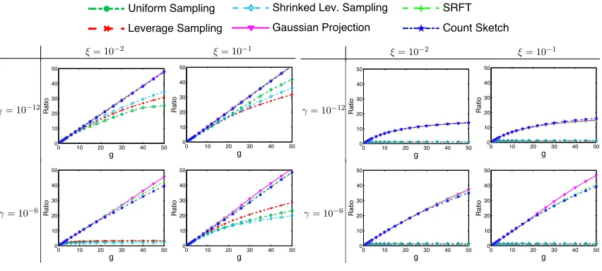
Figure 4: An empirical study of model averaging from the optimization perspective. The
x-axis isg, i.e., the number of models that are averaged. In 4(a), they-axis is the ratio (log-scale) defined in (10). In 4(b), they-axis is the ratio (log-scale) defined in (11). Here γ is the regularization parameter and ξ is the standard deviation of the Gaussian noise.
as measured by the objective function value. For the three random projection methods, the growth rate of this ratio is almost linear in g. In Figure 4(a), we observe that the regularization parameter γ affects the ratio (10). The ratio grows faster when γ = 10−12 than when γ = 10−6. This phenomenon is not explained by our theory.
Theorem 8 shows that for large sketch size s, e.g., Gaussian projection with s= ˜O d
,
f(wh)−f(w?) ≤ β2g +2 kyk22
n −f(w ?),
whereβ = kXk22
kXk2 2+nγ
≤1. In Figure 4(b), we plot the ratio
f(wh [1])−f(w
?)
f(wh
[g])−f(w?)
(11)
againstg. Rapid growth of this ratio indicates that model averaging is highly effective. Our empirical results indicate that the growth rate of this ratio is moderately rapid for very small g and very slow for large g.
4.5 Model Averaging: Statistical Perspective
Sketched Ridge Regression g 050 Variance 10-6 10-5 10-4 Uniform Sampling Leverage Sampling
Shrinked Lev. Sampling
Gaussian Projection SRFT Count Sketch Optimal Solution g 050 Variance 10-6 10-5 10-4 Uniform Sampling Leverage Sampling
Shrinked Lev. Sampling
Gaussian Projection SRFT Count Sketch Optimal Solution g 050 Variance 10-6 10-5 10-4 Uniform Sampling Leverage Sampling
Shrinked Lev. Sampling
Gaussian Projection SRFT Count Sketch Optimal Solution 0 0.51 10-12 Uniform Sampling Leverage Sampling
Shrinked Lev. Sampling
Gaussian Projection
SRFT
Count Sketch
Optimal Solution
Figure 21: .
22
s= 1,000 s= 5,000
= 10 12
0 10 20 30 40 50 10−5
10−4
10−3
10−2 10−1
g
Variance
0 10 20 30 40 50 10−5
10−4 10−3 10−2
g
Variance
= 10 6
0 10 20 30 40 50 10−6
10−5
10−4
10−3
g
Variance
0 10 20 30 40 50 10−6
10−5
10−4
g
Variance
Figure 3: avg var nb classical
h
4
(a)The variance var(wc
[g]).
s= 1,000 s= 5,000
= 10 12
0 10 20 30 40 50 0 10 20 30 40 50 g Ratio
0 10 20 30 40 50 0 10 20 30 40 50 g Ratio
= 10 6
0 10 20 30 40 50 0 10 20 30 40 50 g Ratio
0 10 20 30 40 50 0 10 20 30 40 50 g Ratio
Figure 4: avg varratio nb classical
h
5
(b)The ratio var(w
c [1]) var(wc
[g])
.
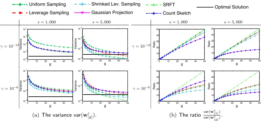
Figure 5: An empirical study of the variance of classical sketch with model averaging. The
x-axis is g, i.e., the number of models that are averaged. In 5(a), the y-axis is the variancevar(w[cg]) (log scale) defined in Theorem 9. In 5(b), they-axis is the ratio var(w
c [1])
var(wc [g])
. Hereγ is the regularization parameter ands is the sketch size.
g 050 Variance 10-6 10-5 10-4 Uniform Sampling Leverage Sampling
Shrinked Lev. Sampling
Gaussian Projection SRFT Count Sketch Optimal Solution g 050 Variance 10-6 10-5 10-4 Uniform Sampling Leverage Sampling
Shrinked Lev. Sampling
Gaussian Projection SRFT Count Sketch Optimal Solution g 050 Variance 10-6 10-5 10-4 Uniform Sampling Leverage Sampling
Shrinked Lev. Sampling
Gaussian Projection
SRFT
Count Sketch
Optimal Solution
Figure 22: .
23
1 10 20 30 40 50
1 1.5 2 2.5 3 3.5 4 g Ratio
(a)s= 1,000
1 10 20 30 40 50
1 1.5 2 2.5 3 3.5 4 g Ratio
(b) s= 2,000
1 10 20 30 40 50
1 1.5 2 2.5 3 3.5 4 g Ratio
(c) s= 5,000
Figure 5: avg biasratio nb hessian
h
Figure 6: An empirical study of the bias of Hessian sketch with model averaging. Thex-axis isg, the number of models being averaged; they-axis is the ratio (12).
and the bias and variance bias(wc
[g]),var(wc[g]) and bias(wh[g]), var(w[hg]) of, respectively, the
model averaged classical sketch solution and the model averaged Hessian sketch solution according to Theorem 9.
Wang, Gittens, and Mahoney
4.5.1 Classical Sketch
Theorem 10 indicates that for large enough s, e.g., Gaussian projection with s = ˜O d 2
, with high probability
bias(wc [g])
bias(w?) ≤1 + and
var(wc [g])
var(w?) ≤ ns
q 1+
h + 2
,
where h= min{g, Θ(n
s)}. This result implies that model averaging decreases the variance
of classical sketch without significantly changing the bias. We conduct experiments to verify this point.
In Figure 5(a) we plot the variance var(wc[g]) against g; the variance of the optimal solutionw?is depicted for comparison. Clearly, the variance drops asggrows. In particular,
when s is big (s = 5,000) and g exceeds ns (= 1005,000,000 = 20), var(wc[g]) can be even lower thanvar(w?).
To more clearly decrease the impact of model averaging on the variance, in Figure 5(b)
we plot the ratio var(w
c [1])
var(wc [g])
against g. According to Theorem 10, this ratio grows linearly in
g when s is at least ˜O(dg), and otherwise is sublinear in g. This claim is verified by the empirical results in Figure 5(b).
Whenbias(w[cg]) is plotted as a function ofg, the curves are almost horizontal, indicating that, as expected, the bias is insensitive to the number of models g. We do not show such plots because these nearly horizontal curves are not interesting.
4.5.2 Hessian Sketch
Theorem 11 indicates that for large enough s, e.g., Gaussian projection with s = ˜O d 2
, the inequalities
bias(wh [g])
bias(w?) ≤ 1 ++
√g +2kXk22
nγ and
var(wh [g])
var(w?) ≤ 1 +
hold with high probability. That is, model averaging improves the bias without affecting the variance. The bound
bias(wh
[g])−bias(w
?)
bias(w?) ≤ +
√g +2kXk22
nγ
indicates that if nγ is much smaller than kXk2
2 and ≤ √1g, or equivalently, s is at least
˜
O(dg), then the ratio is proportional to √g.
To verify Theorem 11, we set γ very small—γ = 10−12—and vary sand g. In Figure 6
we plot the ratio
bias(wh
[1])−bias(w?)
bias(wh
[g])−bias(w?)
, (12)
by fixing γ = 10−12 and varying s and g. The theory indicates that for large sketch size s= ˜O(dg2), this ratio should grow nearly linearly ing. Figure 6 shows that only for large
sand very small g, the growth is near linear in g; this verifies our theory. When we similarly plot var wh
[g]
against g, we observe that var wh [g]
Sketched Ridge Regression
g(=n
s)
2 100 200 300 400 500 600 700
MSE
101 102 103 104 105 106 107
Classical Sketch Model Averaging Optimal Solution
Figure 7: Prediction performance of classical sketch with and without model averaging on the Year Prediction data set. Thex-axis is g, the number of data partitions, and they-axis is the mean squared error (MSE) on the test set.
5. Model Averaging Experiments on Real-World Data
In Section 1 we mentioned that in the distributed setting where the feature-response pairs (x1,y1),· · · ,(xn,yn) ∈ Rd×m are randomly and uniformly partitioned across g
machines,5classical sketch with model averaging requires only one round of communication, and is therefore a communication-efficient algorithm that can be used to: (1) obtain an approximate solution of the MRR problem with risk comparable to a batch solution, and (2) obtain a low-precision solution of the MRR optimization problem that can be used as an initializer for more communication-intensive optimization algorithms. In this section, we demonstrate both applications.
We use the Million Song Year Prediction data set, which has 463,715 training samples and 51,630 test samples with 90 features and one response. We normalize the data by shifting the responses to have zero mean and scaling the range of each feature to [−1,1]. We randomly partition the training data into gparts, which amounts to uniform row selection with sketch size s= ng.
5.1 Prediction Error
We tested the prediction performance of sketched ridge regression by implementing classical sketch with model averaging in PySpark (Zaharia et al., 2010).6 We ran our experiments using PySpark in local mode; the experiments proceeded in three steps: (1) use five-fold cross-validation to determine the regularization parameter γ; (2) learn the modelw using the selected γ; and (3) use w to predict on the test set and record the mean squared errors (MSEs). These steps map cleanly onto the Map-Reduce programming model used by PySpark.
5. If the samples are i.i.d., then any deterministic partition is essentially a uniformly randomly distributed partition. Otherwise, we can invoke a Shuffleoperation, which is supported by systems such as Apache Spark (Zaharia et al., 2010), to make the partitioning uniformly randomly distributed.
Wang, Gittens, and Mahoney
g(= n s)
0 20 40 60 80 100
0 0.2 0.4 0.6 0.8 1 1.2
γ = 10-12
γ = 10-6
γ = 10-4
γ = 10-2
γ = 10-1
(a) Classical sketch
g(= n s)
0 20 40 60 80 100
0 0.02 0.04 0.06 0.08 0.1
γ = 10-12
γ = 10-6
γ = 10-4
γ = 10-2
γ = 10-1
(b) Classical sketch with model averaging
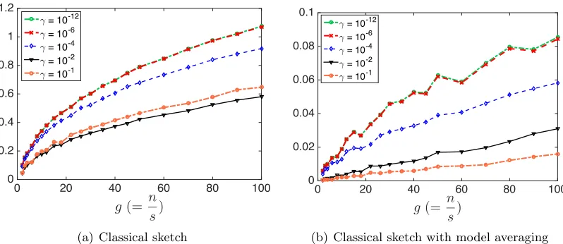
Figure 8: Optimization performance of classical sketch with and without model averaging. Thex-axis isg, the number of data partitions, and they-axis is the ratio kw−w?k2
kw?k
2 .
In Figure 7, we plot the test MSE against g = n
s. As g grows, the sketch size s = n g
decreases, so the performance of classical sketch deteriorates. However classical sketch with model averaging always has test MSE comparable to the optimal solution.
5.2 Optimization Error
We mentioned earlier that classical sketch with or without model averaging can be used to initialize optimization algorithms for solving MRR problems. If w is initialized with zero-mean random variables or deterministically with zeros, thenEkw−w?k2/kw?k2≥1.
Anywwith the above ratio substantially smaller than 1 provides a better initialization. We implemented classical sketch with and without model averaging in Python and calculated the above ratio on the training set of the Year Prediction data set; to estimate the expectation, we repeated the procedure 100 times and report the average of the ratios.
In Figure 8, we plot the average of the ratio kw−w?k2
kw?k
2 against g for different settings of
the regularization parameterγ. Clearly, classical sketch does not give a good initialization unless g is small (equivalently, the sketch size s = ng is large). In contrast, the averaged solution is always close to w?.
6. Sketch of Proof
In this section, we outline the proofs of our main results. The complete details are provided in the appendix. Section 6.1 recaps several relevant properties of matrix sketching. Section 6.2 establishes certain properties of averages of sketches; these results are used to analyze the application of model averaging to the MRR problem. Sections 6.3 to 6.6 provide key structural results on sketched solutions to the MRR problem constructed with or without model averaging.
Sketched Ridge Regression
sketched MRR problem. Table 4 summarizes the dependency relationships among these theorems. For example, Theorem 1, which studies classical sketching from the optimization perspective, is one of our main theorems and is proven using Theorems 12 and 15.
Table 4: An overview of our results and their dependency relationships.
Main Theorems Solution Perspective Prerequisites
Theorem 1 classical optimization Theorems 12 and 15
Theorem 2 Hessian optimization Theorems 12 and 16
Theorem 5 classical statistical Theorems 12, 13, 17, 18
Theorem 6 Hessian statistical Theorems 12 and 19
Theorem 7 classical, averaging optimization Theorems 14 and 20 Theorem 8 Hessian, averaging optimization Theorems 14 and 21 Theorem 10 classical, averaging statistical Theorems 14 and 22 Theorem 11 Hessian, averaging statistical Theorems 14 and 23
6.1 Properties of Matrix Sketching
Our analysis of the performance of solutions to the sketched MRR problem draws heavily on the three key properties defined in Assumption 1. Theorem 12 establishes that the six sketching methods considered in this paper indeed enjoy the three key properties under certain conditions. Finally, Theorem 13 establishes the lower bounds of kSk2
2 that are used
to prove the lower bounds on the variance of sketched MRR solutions in Theorem 5.
Assumption 1 Letη, ∈(0,1)be fixed parameters. LetBbe any fixed matrix of conformal shape, ρ= rank(X), andU∈Rn×ρ be an orthonormal basis for the column span ofX. Let S∈Rn×s be a sketching matrix, wheres depends onη and/or. Throughout this paper, we
assume that S satisfies the following properties with a probability that depends on s: 1.1 UTSSTU−I
ρ
2 ≤η (Subspace Embedding Property);
1.2 UTSSTB−UTB 2
F ≤kBk 2
F (Matrix Multiplication Property);
1.3 When s < n,kSk22 ≤ θns for some constant θ (Bounded Spectral Norm Property). The subspace embedding property requires that sketching preserves the inner products between the columns of a matrix with orthonormal columns. Equivalently, it ensures that the singular values of any sketched column-orthonormal matrix are all close to one. The subspace embedding property implies that, in particular, the squared norm of Sx is close to that ofx for any n-dimensional vector in a fixed ρ-dimensional subspace. A dimension counting argument suggests that since Sx is an s-dimensional vector, its length must be scaled by a factor ofpn
s to ensure that this consequence of the subspace embedding property
holds. The bounded spectral norm property requires that the spectral norm ofSis not much larger than this rescaling factor ofpn
s.
Wang, Gittens, and Mahoney
Table 5: The two middle columns provide an upper bound on the sketch size sneeded to satisfy the subspace embedding property and the matrix multiplication property, respectively, under the different sketching modalities considered; the right column lists the parameterθwith which the bounded spectral norm property holds. These properties hold with constant probability for the indicated values of s. Here τ is defined in (5) and reflects the quality of the approximation of the leverage scores ofU;µis the row coherence of U. For Gaussian projection and CountSketch, the small-onotation is a consequence of s=o(n).
Sketching Subspace Embedding Matrix Multiplication Spectral Norm
Leverage s=O τ ρ η2log
ρ δ1
s=O τ ρ δ2
θ=∞
Uniform s=O µρ η2log
ρ δ1
s=O µρ δ2
θ= 1 Shrinked Leverage s=O τ ρ
η2log ρ δ1
s=O τ ρ δ2
θ= 2 SRHT s=O ρ+logn
η2 log ρ δ1
s=O ρ+logn δ2
θ= 1 Gaussian Projection s=O ρ+log(1/δ1)
η2
s=O ρ δ2
θ= 1 +o(1) w.h.p. CountSketch s=O ρ2
δ1η2
s=O ρ δ2
θ= 1 +o(1) w.h.p.
The third assumption is new, but Ma et al. (2015); Raskutti and Mahoney (2016) demonstrated that some sort of additional condition is necessary to obtain strong results from the statistical perspective.
Remark 3 We note that UTU = I
ρ, and thus Assumption 1.1 can be expressed in the
form of an approximate matrix multiplication bound (Drineas et al., 2006a). We call it the Subspace Embedding Property since, as first highlighted in Drineas et al. (2006b), this subspace embedding property is the key result necessary to obtain high-quality sketching algorithms for regression and related problems.
Theorem 12 shows that the six sketching methods satisfy the three properties whensis sufficiently large. In particular, Theorem 12 shows that for all the sketching methods except leverage score sampling,7 kSk22 has nontrivial upper bound. This is why Theorems 5 and 10 do not apply to leverage score sampling. This fact can also be viewed as a motivation to use shrinked leverage score sampling. We prove Theorem 12 in Appendix A.
Theorem 12 Fix failure probability δ and error parameters η and ; set the sketch size s
as Table 5. Assumption 1.1 is satisfied with probability at least 1−δ1. Assumption 1.2 is
satisfied with probability at least 1−δ2. Assumption 1.3 is satisfied either surely or with
high probability (w.h.p.); the parameter θ is indicated in Table 5.
Theorem 13 establishes lower bounds on kSk22, and will be applied to prove the lower bound on the variance of the classical sketch. From Table 6 we see that the lower bound for
7. If one leverage score approaches zero, then the corresponding sampling probabilitypigoes to zero. By the definition of S, the scale factor √1
spi goes to infinity, which makeskSk
2
2 unbounded. The shinked
Sketched Ridge Regression
(shrinked) leverage score sampling is not interesting, because µ can be very large. This is why Theorem 5 does not provide a lower bound for shrinked leverage score sampling. We prove Theorem 13 in Appendix A.
Table 6: Lower bounds onϑfor the sketching modalities (ϑis defined in Theorem 13). The shrinked leverage score sampling is performed using the row leverage scores of a matrixX∈Rn×d, and µis the row coherence ofX.
Uniform ϑ= 1
Leverage ϑ≥ 1
µ
Shrinked Leverage ϑ≥ 2
1+µ
SRHT ϑ= 1
Gaussian Projection ϑ≥1−o(1) w.h.p. CountSketch ϑ≥1−o(1) w.h.p.
Theorem 13 (Semidefinite Lower Bound on the Sketching Matrix) When s < n,
STS ϑn
s Is holds either surely or with high probability (w.h.p.), where Table 6 provides the
applicableϑ for each sketching method.
Remark 4 Let p1,· · ·, pn be an arbitrary set of sampling probabilities. By the definition
of the associated sampling matrix S∈Rn×s, the non-zero entries of S can be any of √1 spi, for i∈[n].
For leverage score sampling, since the smallest sampling probability can be zero or close, and the largest sampling probability can be close to one, kSk2
2 has no nontrivial upper or
lower bound.8 It is because minipi can be close to zero and maxipi can be large (close to
one).
For shrinked leverage score sampling, becauseminipi is at least 21n,kSk22 has a nontrivial
upper bound; but as in the case of leverage score sampling, since maxipi can be large, there
is no nontrivial lower bound onkSk22.
6.2 Matrix Sketching with Averaging
Assumptions 1.1 and 1.2 imply that sketching can be used to approximate certain matrix products, but what happens if we independently drawg sketches, use them to approximate the same matrix product, and then average the g results? Intuitively, averaging should lower the variance of the approximation without affecting its bias, and thus provide a better approximation of the true product.
To justify this intuition formally, let S1,· · · ,Sg ∈ Rn×s be sketching matrices and A
and B be fixed conformal matrices. Then evidently
1 g
g
X
i=1
ATSiSTiB = A T
SSTB,
8. In our application, nontrivial bound meanskSk2