Optimally-Smooth Adaptive Boosting and
Application to Agnostic Learning
Dmitry Gavinsky [email protected]
Department of Computer Science University of Calgary
Calgary, Alberta, Canada, T2N 1N4
Editor: Dana Ron
Abstract
We describe a new boosting algorithm that is the first such algorithm to be both smooth and adaptive. These two features make possible performance improvements for many learning tasks whose solutions use a boosting technique.
The boosting approach was originally suggested for the standard PAC model; we analyze pos-sible applications of boosting in the context of agnostic learning, which is more realistic than the PAC model. We derive a lower bound for the final error achievable by boosting in the agnostic model and show that our algorithm actually achieves that accuracy (within a constant factor).
We note that the idea of applying boosting in the agnostic model was first suggested by Ben-David, Long and Mansour (2001) and the solution they give is improved in the present paper. The accuracy we achieve is exponentially better with respect to the standard agnostic accuracy parameterβ.
We also describe the construction of a boosting “tandem” whose asymptotic number of itera-tions is the lowest possible (in bothγandε) and whose smoothness is optimal in terms of ˜O(·). This allows adaptively solving problems whose solution is based on smooth boosting (like noise tolerant boosting and DNF membership learning), while preserving the original (non-adaptive) solution’s complexity.
1. Introduction
Boosting is a learning method discovered by Schapire (1990). It proves computational equiva-lence between two learning models: the model of distribution-free (strong) PAC-learning and that of distribution-free weak PAC-learning (the PAC-model was first introduced by Valiant, 1984; the strong and the weak cases were distinguished by Kearns and Valiant, 1994). This (theoretical) equiv-alence between the two models may be used to solve various problems in the domain of Learning Theory—a number of such problems are currently known whose “strong” solution was achieved by initially constructing a weak learner and then applying a boosting algorithm.
It turns out that the boosting approach, originally developed for the standard PAC model, may be adapted to other more or less similar learning models. For example, the solution suggested in Jackson (1997) for the DNF learning problem is partially based on a previously known boosting algorithm, adapted for the uniform model with allowed membership queries.
Recently Ben-David, Long and Mansour (2001) have shown that the boosting approach may also be applied in the model of agnostic learning, which is in a sense “more practical” than PAC (see Subsection 1.1.3 for model description).
In this paper we construct a boosting algorithm whose requirements for some resources are “optimally modest”; as a result, this algorithm may be used in a number of “near-PAC” learning models, achieving the optimal performance.
1.1 Learning Models
All the models considered in this paper have one feature in common: a learner always communicates with a D-oracle which produces examples(x,f(x)), where f is the target function and x is chosen from the domain X according to the distribution D.
In this paper we will always assume that f is binary-valued to{−1,1}. We will sometimes use as a complexity parameter a measure of the representation size of f , which we denote by I(f)(its definition depends on the target class and is usually clear from the context). Therefore the difference between the following models lies in the requirements for the learner’s complexity and accuracy.
1.1.1 PAC LEARNING (STRONG)
The target function f is assumed to come from some hypotheses class C. The learner receives parameters ε and δ; its goal is to produce with probability at least 1−δa binary hypothesis hfin, satisfying:
εhfin,Pr
D[hfin(x)6= f(x)]≤ε.
The time complexity of the learner should be polynomial in 1/ε, log(1/δ)and I(f). (Sometimes
δis referred to as a confidence parameter.)
1.1.2 PAC LEARNING (WEAK)
The target function f is assumed to come from some hypotheses class C. The learner receives a parameterδ; its goal is to produce with probability at least 1−δa hypothesis hfin, satisfying:
γhfin,E
D[h(x)·f(x)]≥γmin,
whereγmindecreases inversely polynomially in I(f)(we will use the notationγhto denote the value of ED[h(x)·f(x)]for any real-valued h defined over X ). In the context of weak PAC learning we will not require the produced hypothesis to be binary (it may be real-valued to[−1,1]).
The time complexity of the learner should be polynomial in I(f)and log(1/δ).
1.1.3 AGNOSTIC LEARNING
F to be used for learning. For any target function f , the best possible accuracy a hypothesis from F can achieve is either equal or infinitesimally close to
err
D(F),hinf0∈F n
Pr D
h0(x)6= f(x)o.1
The learner receives a parameterδ and has to produce with probability at least 1−δa binary hypothesis hfin, satisfying:
εhfin≤err
D(F) +β,
for someβannounced a priori. A learner satisfying this is called aβ-optimal learner.
We do not define a general notion of agnostic learning efficiency here; for a detailed overview of the agnostic learning model, see Kearns, Schapire and Sellie (1994).
1.2 Boosting
A boosting algorithm B is supplied with an auxiliary algorithm W L (the weak learner). B commu-nicates with W L, in a sequence of sessions: During session i B chooses a distribution Diover X and emulates for W L a Di-oracle, answering according to the target function f . In response W L has to learn f w.r.t. Di, each session ends when W L constructs its hypothesis.
We will denote the total number of performed boosting sessions by T and the weak learner’s response to Diby hi. We will sometimes refer to individual sessions as “iterations”.
The boosting algorithm itself “faces” some target distribution D, according to which it receives instances from the oracle. After the T ’th session is finished, B produces its final hypothesis hfin whose accuracy w.r.t. D is higher than the accuracies of the received weak hypotheses (w.r.t. corre-sponding Di-s).
When the boosting is performed in the PAC model, the weak learner is usually a weak PAC-learner and the booster itself is required to satisfy the strong PAC requirements (see Subsection 1.1.1). In this case the booster is considered efficient when its complexity is polynomial in theγmin param-eter of W L, as well as in standard PAC complexity paramparam-eters. Note that when W L is an efficient weak PAC learner (i.e., γmin is inverse-polynomial low), the whole tandem B+W L constitutes an efficient strong PAC learner.
For the case of agnostic model (see Subsection 1.1.3) we will derive efficiency requirements for both B and W L later in the paper. (Since the PAC model is “more natural” for boosting, we will describe and analyze our algorithm as a PAC booster, and then we will separately consider its usage under agnostic settings.)
1.2.1 BOOSTING BYSAMPLING VERSUS BOOSTING BYFILTERING
In this paper we consider two boosting modes: boosting by sampling and boosting by filtering. Boosting by sampling means that the learning is performed in two stages. In the first stage the algorithm collects a sufficient number of learning examples (i.e., a subset S⊂X together cor-responding values of f ) by repeatedly calling the oracle. In the second stage the booster performs learning over this collection of examples only. The training sample S is of polynomial size.
The booster’s goal is to achieve some required accuracy over the training set (which is often the absolute accuracy, so that the hypothesis coincides with f for each x∈S). Then information-theoretic techniques like VC theory (Vapnik, 1982) and Occam’s Razor (Blumer, Ehrenfeucht, Haussler and Warmuth, 1989) may be applied to measure the overall accuracy w.r.t. D of the same hypothesis.
Of course, the hypothesis may be not accurate over whole X even if it is correct over S. Such “switching” from sub-domain S to whole X is sometimes called generalization, and the additional error introduced by generalization is called a generalization error.
In contrast, when boosting by filtering the booster takes the whole set of instances as its learning domain. The examples received by the booster from the PAC-oracle are not stored, but are “filtered”: each example is either forwarded to W L or rejected (i.e., is not used at all).
This approach has two obvious advantages over boosting by sampling: the space complexity is reduced (the examples are not stored) and no generalization error is introduced. At the same time, the analysis and the algorithm itself become slightly more complicated, because now the booster cannot get exact statistics by running through all the instances of the domain and needs to use some estimation schemes (based on various statistical laws of large numbers, like the Chernoff bound).
Among the possible reasons for using boosting by sampling is that the booster is not smooth: In general, a distribution which is not polynomially near-D cannot be efficiently simulated using repeated calls to a D-oracle, when X is superpolynomially large.
1.2.2 SMOOTHBOOSTING ANDADAPTIVE BOOSTING
In this paper we consider two special features of boosting algorithm: smoothness and adaptiveness. The term “adaptiveness” means that the algorithm doesn’t require a priori lower bound for γi; instead the algorithm “takes advantage” of each single weak hypothesis, as good as it is. More for-mally, while a non-adaptive booster has its complexity bounds polynomial in 1/min{γhi|1≤i≤T},
adaptive algorithm’s running time is polynomial in
1/ E
1≤i≤T[poly(γhi)].
(For example, we will derive complexity bounds for our algorithm in terms of 1/E1≤i≤T
γ2 i
.) The term “smoothness” means that the distributions Diemulated by the booster do not diverge dramatically from the target distribution D of the booster itself. To measure the “smoothness” of a distribution Di, we define a smoothness parameter:
αi,sup
x∈X Di(x)
D(x).
We define a smoothness parameter for a boosting algorithm as sup of possible smoothness param-eters of distributions emulated by it. A boosting algorithm with smoothness parameter α will be calledα-smooth.
1.3 Our Results
In this paper we construct a boosting algorithm called AdaFlat, which is optimal from several points of view. We show that AdaFlat is adaptive and near-optimally smooth (within a constant multiplicative factor of 2).
Let us consider a variation of the above adaptiveness notation: Call a booster output-adaptive if the size of the final hypothesis it produces is adaptive (i.e., is bounded above by a polynomial in 1/E1≤i≤T[poly(γhi)]). For notation clarity we will sometimes refer to the “usual” adaptiveness (as
defined above) as time-adaptiveness.
If the size of the final hypothesis depends polynomially on γhi-s, then time-adaptiveness
nat-urally implies output-adaptiveness. To the best of our knowledge, this is the case for all known boosting algorithms.
Claim 1 If the size of the final hypothesis depends polynomially onγhi-s, then smoothness is
essen-tial for performing adaptive boosting over a superpolynomially large domain.
Proof of Claim 1 The booster is output-adaptive, assume that it is not smooth.
On the one hand, non-smoothness obliges to use boosting by sampling. On the other hand, for an output-adaptive booster it is not in general possible to bound from above “adaptively” the size of the final hypothesis before the boosting process ends.
In order to fix the size of the learning sample S so that the final error (after generalization) would be at most ε, it is essential to have an upper bound for the size of the final hypothesis (e.g., see Vapnik 1982 and Blumer, Ehrenfeucht, Haussler and Warmuth 1989 for overview of generalization techniques).
Because the size of the learning domain must be fixed before boosting by sampling starts and at that time we do not have an adaptive upper bound for the size of the final hypothesis, we have to use a learning sample of adaptive size, which turns the boosting algorithms itself into non-time-adaptive.
Claim 1
To the best of our knowledge, AdaFlat is the first smooth adaptive booster.
An algorithm MadaBoost constructed by Domingo and Watanabe (2000) is smooth, but it is adaptive only for a non-increasing sequence of weak hypotheses accuracies (i.e., whenγhi+1 ≤γhi
for 1≤i≤T−1). Besides, their result applies only to the case of binary-valued weak hypotheses, which seems to produce some difficulties when Fourier spectrum approach is used for weak learning (Mansour, 1994, Blum, Furst, Jackson, Kearns, Mansour and Rudich, 1994, Bshouty, Jackson and Tamon, 1999).
Another similar result was achieved by Bshouty and Gavinsky (2001): their algorithm is smooth and output-adaptive, but not time-adaptive: While their algorithm makes adaptive number of boost-ing iterations and constructs final hypothesis of adaptive size, the time complexity of each iteration depends upon the value ofγmin(which should be provided before the boosting starts).
We show that AdaFlat may be used in the framework of agnostic learning. We derive a lower bound for the final error achievable by agnostic boosting; we show that our algorithm achieves that accuracy (within a constant factor of 2). Our upper bound on the final error is
1
whereζis any real so that the time complexity of the solution is polynomial in 1/ζ.
The idea of applying boosting in the agnostic model is due to Ben-David, Long and Mansour (2001). Our result is an exponential improvement w.r.t.βover the solution suggested in Ben-David, Long and Mansour (2001), whose error is upper bounded by
1
1/2−βerrD(F)
2(1/2−β)2/ln(1/β−1)
+ζ.
(In particular, this answers an open question posed in Ben-David, Long and Mansour 2001.) Algorithm AdaFlat performs the lowest possible asymptotic number of boosting iterations in terms ofγ.
Next we construct a “boosting tandem”, consisting of AdaFlat “joined” with another boosting algorithm (this approach was first used by Freund (1992) and since then has become very popular for constructing boosting algorithms). The underlying idea is to use one booster (AdaF lat, in our case) to boost hypotheses from “weak” accuracy 12+γto some fixed accuracy12+const,and then to amplify(12+const)-accurate hypotheses to 1−εusing another boosting algorithm. This approach is used when the first booster is more efficient in terms ofγand the second one is more efficient in terms ofε.
Moreover, since adaptiveness means certain behavior of a booster w.r.t. the parameter γand AdaFlat is used as the ‘bottom level” for the tandem, the whole construction remains adaptive.
Naturally, the final hypothesis structure of the tandem is more complicated. On the other hand, using this approach we achieve the lowest possible asymptotic number of boosting iterations both inγand inε, and also the lowest possible smoothness factor in terms of ˜O.2
Since our tandem algorithm is also adaptive, it may be used in order to solve adaptively and with optimal number of iterations various boosting tasks, including those requiring that the boosting algorithm be smooth.
2. Preliminaries
For simplicity, in our analysis of boosting schemes we will not allow W L to fail.
2.1 Agnostic Boosting Approach
The main idea standing behind agnostic boosting is as follows: suppose we are given aβ-optimal learning algorithm; it will be used as a weak learner and therefore is referred to by W L.
Consider some target distribution D. By definition, the weak learner being executed “in a straightforward manner” must provide a(1−errD(F)−β)-accurate hypothesis in the worst case. Let us modify slightly the target distribution thus achieving a new distribution Diof smoothnessαi (measured w.r.t. D). Obviously, it holds that
err Di
(F)≤αi·err D(F),
and W L must provide a hypothesis hiwhose error isαi·errD(F) +β,in the worst case.
If distribution Diwas produced by a boosting algorithm on stage i, then using boosting notation we may write:
αi·err
D(F) +β≥εi= 1 2−γi,
which leads to
γi≥
1
2−β−αi·errD(F). (1)
While Ben-David, Long and Mansour (2001) mainly considered agnostic learning in the context of boosting by sampling, our result applies equally to both boosting by sampling and boosting by filtering. In fact, it seems that the main difficulty lies in constructing a weak learner; possible solutions for this determine the applicability and the efficiency of the boosting methods. Some examples of “agnostic weak learners” may be found in Ben-David, Long and Mansour (2001).
3. Optimally-Smooth Adaptive Boosting
In this section we construct a booster working by sampling and in Section 5 we build a modification of the algorithm which works by filtering. For the construction of AdaFlat we modify another algorithm, first introduced by Impagliazzo (1995) in a non-boosting context and later recognized as a boosting algorithm by Klivans and Servedio (1999).
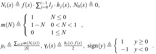
Algorithm AdaFlat is represented in Figure 1, the following notation is used:
Ni(s), f(s)·∑ij−=10lj·hj(s), N0(s),0,
m(N),
1 N≤0
1−N 0<N<1
0 1≤N
,
µi,∑s∈Sm(Ni(s))
|S| ,γi(s),
hi(s)·f(s)
2 , sign(y),
1 y≥0
−1 y<0 .
When the domain S is of polynomial size, simulation of Di-s is straightforward. Note that the number of iterations performed by the algorithm defines the number of weak hypotheses combined in a final hypothesis.
AdaFlat(W L,S,ε) 1. set: i=0
2. while Prs∈S[hfin(s)6= f(s)]≥ε 3. define: Di(s),∑m(Ni(s))
s∈Sm(Ni(s))
4. call W L, providing it with distribution Di; denote the returned weak hypothesis by hi 5. set: γi=∑s∈SDi(s)·γi(s)
6. set: li=2µiγi
7. define: hfin(s),sign ∑ij=0lj·hj(s)
8. set: i=i+1 9. end-while
10. Output the final hypothesis hfin
3.1 AdaFlat’s Analysis
Claim 2 Algorithm AdaF lat executed with parameters(W L,S,ε)performs
T ≤ ε
−2 4 E0≤i<T
γ2 i
(2)
boosting iterations and produces a final hypothesis which is accurate over S and possesses the structure of a weighted majority vote of T weak hypotheses. The smoothness parameter of AdaFlat satisfies:
α≤ε−1. (3)
Proof of Claim 2 Define the following reward function:
B(N),
N N≤0 N−N22 0<N<1 1
2 1≤N
.
As follows from a second-order Taylor expansion, for any c∈R it holds:
B(N+c)≥B(N) +dB
dN·c+inf B
00(N)·c2
2,
where B00(N),min{dNdB·dN2+, dB
2
dN·dN−}.By noting that m(N) = dB
dN,we get:
B(N+c)≥B(N) +m(N)·c−c 2 2.
Further, denote:
ci(s),Ni(s)−Ni−1(s) =li·hi(s)·f(s) =2liγi(s), Bi,∑s∈SB(Ni(s))
|S| ,
∆i
B,Bi+1−Bi. Consequently,
∆i
B ≥∑s∈S
m(Ni(s))·ci(s) |S| −
∑s∈Sc2i(s)
2|S|
≥2li∑s∈∑Sm(Ni(s))·γi(s)
s∈Sm(Ni(s)) ·µi−
l2
i
2 =2liγiµi−li2
2 , and using the expression set for liby AdaF lat, we get:
∆i
B≥2γ2i ·µ2i. (4) Since B(N)≤12,the last inequality leads to
T ≤ 1
4 E0≤i<T
γ2 i ·µ2i
We can see that the number of iterations T depends on E0≤i<T
γ2 i
(rather than on min20≤i<T[γi]), and therefore the algorithm is adaptive.
Next, it holds that 1
αi =
1
|S|· 1
maxs∈SDi(s) =
µi
maxs∈Sm(Ni(s)).
(6)
But the algorithm would stop as soon as the error of the last constructed hfinbecomes less or equal toε, so for each i it holds that
argmax s∈S
m(Ni(s)) =min
s∈S Ni(s)≤0,
and therefore maxs∈Sm(Ni(s)) =1. At the same time, this means that µi≥εas long as AdaFlat continues to run (which follows from the definition of µi). Applying this to (6), we get
α−1
i =µi≥ε, (7) which leads to (3).
Combining (7) with (5), we receive statement (2), and the result follows.
Claim 2
4. Agnostic Boosting
In this section we apply AdaF lat to agnostic boosting. (We refer to AdaFlat which works by sampling and not to AdaFlatFilt introduced in Section 5; however, algorithm AdaF latFilt may be used for agnostic boosting as well.) As a result, we achieve upper bound on final error of
1
1/2−βerrD(F) +ζ,
whereζis any real, so that the time complexity of the solution is polynomial in 1/ζ, as well as in other standard complexity parameters.
The analysis of our new application is straightforward: Combining (1), (4) and (7) gives us that:
∆i B≥2
γi αi
2
≥(ε 1 2−β
−errD(F))2, T ≤14 ε 12−β−errD(F)
−2
,
ε≤ 2√1T+errD(F)
1
2−β .
That is, applying AdaFlat to the task of agnostic boosting allows to get a hypothesis which
errD(F)
1 2−β
+ζ -approximates the target concept. For that, AdaFlat needs to perform
T ≤1 4
ζ·
1 2−β
−2
Recall that if we straightly apply W L, we get a(errD(F) +β)-approximation. Therefore, our approach actually amplifies W L if and only if
err
D(F)<β· 1−2β 1+2β.
Note that asymptotic evaluation would work well for the number of iterations needed, but is not sufficient for the smoothness estimation (3). That is because the smoothness property determines the “base” for the final error expression
errD(F)
1 2−β
,which seems to be rather “hard” (in particular, cannot be decreased simply by performing a larger number of boosting iterations). The same thing holds regarding the parameterβ.
In Section 6 we show that AdaFlat (and AdaFlatFilt) are near-optimally smooth up to the con-stant multiplicative factor of 2, therefore the final hypothesis has half the best possible relative correspondence with the target for the agnostic boosting approach.
5. Boosting Using Filtering
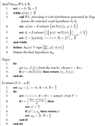
Algorithm AdaF latFiltis shown in Figure 2. Note that the algorithm receives confidence parameter
δ. Recall that now the target distribution is D itself and the instance space is{(x,f(x))|x∈X}. The algorithm has two subroutines: Digen which is used to produce examples for W L and Evaluate(V,b−a,δ) which, with probability δat least, returns a value µ0 s.t. |µ0−E[V]| ≤ E[5V] when V receives values from [a,b]and E[V]6=0.The latter subroutine is based on the Chernoff bound, its time complexity is
O
(b−a)2·ln(δ−1)·ln((E[V])−1) (E[V])2
.
5.1 AdaFlatFilt’s Analysis
Denote by T[W L]the time complexity of W L running over the instance space X , and by Q[W L]the corresponding query complexity (i.e., the number of requested examples).
The time and query complexity bounds introduced by the following claim are not tight, they are reconsidered and improved in Subsection 5.2.
Claim 3 Suppose that algorithm AdaFlatFilt is executed with parameters (W L,ε,δ). Then with probability at leastδthe following statements hold:
- The algorithm performs
T ≤ 3
4ε2·E 0≤i<T
γ2 i
(8)
boosting iterations.
- The algorithm produces a final hypothesis possessing the structure of a weighted majority vote of T weak hypotheses whose prediction error over the learning domain (X ) isεat most.
- The smoothness parameter of AdaFlatFilt satisfies
AdaFlatFilt(W L,ε,δ) 1. set: i=0, δ0= δ2 2. while µ0i(m)≥45ε
3. call W L, providing it with distribution generated by Digen; denote the returned weak hypothesis by hi
4. set: µ0i(m) =Evaluate
m(Ni(s))|s∼D,1,δ2i
5. set:γ0i=Evaluate
γi(s)·m(Ni(s))
s∼D,1, δi
2
6. set: li0=2µi0(m)γ0i, i=i+1, δi=32l02i−1·δ 7. end-while
8. define: hfin(s),sign
∑i
j=0l0j·hj(s)
9. Output the final hypothesis hfin
Digen
1. do
2. get(xj,f(fj))from the oracle; choose r∼U0,1 3. if(r<m(Ni(s)))then return(xj,f(xj)) 4. end-do
Evaluate(V,b−a,δ)
1. set: µg= 12, i=0, σ=0,δ=δ2
2. do
3. set: i=i+1,σ=σ+<sample f rom V >
4. if i=
l18(b−a)2ln(2
δ)
µ2
g m
then
5. set: µ0= σi
6. if|µ0| ≥µgthen return µ0 7. set: µg=µ2g, δ= δ2
8. end-if
9. end-do
Figure 2: The AdaFlatFilt(W L,ε,δ)hypothesis boosting algorithm.
- The query complexity of the algorithm is
˜ O ε
−1·Q[W L] +E 0≤i<T
γ−2 i
+ε−2
ε2·E
0≤i<T γ2 i ! . (9)
- The time complexity of the algorithm is
˜ O ε
−1·Q[W L] +T[W L] +E 0≤i<T
γ−2 i
+ε−2
ε2·E
Proof of Claim 3 Notice that AdaFlatFilt is smooth as well, Equation (3) still holds.
Now we calculate the overall number T of iterations (by adjusting slightly the analysis given for AdaFlat in Subsection 3.1). Start by assuming that all the estimations performed by Evaluate (lines 4 and 5 of AdaFlatFilt) are accurate within a relative factor of 15 (i.e., within 20% accuracy), later we show that the probability of this event is 1−δat least.
That is, suppose that during the i’th iteration the assumption holds; therefore, the resulting value received for l0i estimates within a relative factor of12 the “real” value of li, as defined before. In this case, Equation (4) can be rewritten as follows:
∆i B≥
3 2·γ
2 iµ2i.
The halting condition µ0i(m)<45εguarantees, on the one hand, that the final error is smaller than
ε(i.e., AdaFlatFilt is accurate), and, on the other hand, that throughout the iterations µi is at least 2ε
3. This leads to (8).
Next, we prove the following statement: the probability that our estimations accuracy assump-tion fails during stage 0 and k following stages is(12+Bk)·δat most. Note that, under the assump-tion of statement correctness for stages 0−k, the value ofδk+1set in line 6 is not greater than∆kB·δ, and the result follows. As it is always true that Bk≤12, the failure probability is bounded from above byδand AdaF latFiltsatisfies the confidence requirement.
It remains to evaluate the time and number of queries consumed by each boosting iteration (under the estimations accuracy assumption). It holds for i≥1 that δi>151ε2γ2i−1δ,therefore two calls to Evaluate take
O ln(δ−1ε−1γi−−11)· ln(γ
−1 i )
γ2 i
+ln(εε2−1) !!
.
Getting a single example from Digen takes in average
1 µi ≤ε
−1
time, therefore the (average) query complexity of a single call to W L is
O ε−1·Q[W L].
The resulting query complexity of a single boosting iteration is
O ε−1·Q[W L] +ln(δ−1ε−1γ−i−11)· ln(γ
−1 i )
γ2 i
+ln(εε2−1) !!
, (11)
and the time complexity is
O ε−1·Q[W L] +T[W L] +ln(δ−1ε−1γ−i−11)· ln(γ
−1 i )
γ2 i
+ln(εε2−1) !!
. (12)
In terms of ˜O,these expressions respectively correspond to
˜
queries and
˜
O ε−1·Q[W L] +T[W L] +γ−i 2+ε−2 time needed for the i’th boosting iteration.
Obviously, the case of i=0 will not rise the average iteration complexity resulting from these observations. Combining them with Equation (8) gives the required bounds (9) and (10), and the result follows.
Claim 3
5.2 Implementation Considerations
The complexity bounds (11) and (12) (see the proof of Claim 3) depend on bothγiandγi−1, which may be viewed as a certain kind of “memory”, or a loss of adaptiveness. This effect may be removed by halving δ after each iteration (in line 6), in this case the logarithmic terms are replaced by polynomials “without memory”. To our point of view, the complexity resulting from the “attaching”
δito∆iB−1is better, despite the mentioned weakness (which, in fact, completely disappears in terms of ˜O).
Next, note that ifγi approaches the value of 0 this considerably increases the time needed for Evaluate in order to estimate its value; to avoid this, we may introduce a lower bound for “ac-ceptable” γi-s. B.t.w., the case of negative γi rises no difficulties (it is “turned into positive” by corresponding negative li).
Another consideration may useful as well in this connection. It seems like a very natural as-sumption that W L, while producing a weak hypothesis, is capable to report the received accuracy. In this case, the term of E0≤i<T
γ−2 i
disappears from the complexity bounds: for instance, the time complexity would be bounded by
˜ O ε
−1·Q[W L] +T[W L] +ε−2
ε2·E
0≤i<T
γ2 i
!
.
Further, examples may be “reused” throughout the computation, both for W L teaching and for values estimation.3 Of course, in this case the algorithm requires additional memory of size equal to the query complexity. Assuming that W L reports the accuracies, both storage and query complexity is bounded by
˜
O ε−1·Q[W L] +ε−2.
Notice that our adaptive technique is aimed to minimize the number of performed iterations, from this point of view it is worth to make use of each received weak hypothesis, including those with small |γi|-s. On the other hand, slightly different approach should be used to minimize the overall time and/or query complexity: for example, consider, as described above, setting a lower bound for acceptable|γi|-s in order to avoid “too expensive” mean value estimations.
6. Optimality of AdaFlat and AdaFlatFilt
In this section we consider the smoothness parameter and the number of iterations performed by our algorithms.
Claim 4 The following holds for the algorithms AdaF lat and AdaF latFilt:
- Their smoothness parameters are not higher than two times the minimum required for suc-cessful boosting.
- The asymptotic number of iterations they perform is optimal in terms ofγ.
Proof of Claim 4 The second part of the claim follows from a result by Freund (1995): The number T of iterations of any boosting scheme must satisfy
T =Θ γ−2·lnε−1.
The fact that α≤ε−1 is near-optimal up to the multiplicative factor of 2 becomes clear from the following argument: Consider a general boosting algorithm, suppose that it is not allowed to diverge from the original distribution D by more than
ε−1·(1
2−
1 2γ) =
1−γ
2ε . (13)
Now suppose that the weak learner chooses some region Y ⊂X such that
D(Y) =ε,
and then produces the following hypothesis:
hY=
f(x) i f x∈/Y
−f(x) otherwise .
Note that in this case the region Y should not be chosen randomly. We only require that the booster (which is supposed to be general, i.e., not restricted to a specific weak learner) has no information about Y and therefore must treat this region as a randomly chosen one.
As long as the target distribution for the weak learner has smoothness parameter not greater than (13), the weak learner may repeatedly return the hypothesis hY and still satisfy its specifications.
On the other hand, since form the booster’s point of view the region Y is randomly chosen, the best thing the booster can do is to attach a list of polynomially many points from Y as a “correction” to hY.Since such a correction has, in general, only exponentially small impact, it can be neglected, and the final error may be assumed to be equal to D(Y) =ε.
The maximum smoothness parameter we have allowed is(1−γ)/2ε,and sinceγdecreases poly-nomially as the input size grows, the parameter can be made arbitrary close toε−1/2,as required.
Claim 4
7. Boosting Tandems
by the booster into a polynomially-accurate strong hypothesis, in the boosting tandem model the corresponding evolution is polynomial weak→constant correspondence→polynomial strong. This technique was first used by Freund (1992). Its advantage is that if one algorithm is more efficient in terms ofγand the other in terms ofε, this approach makes use of the “strong sizes” of the both, setting their “weak” parameters to constants.
Naturally, we are interested in preserving the adaptiveness and efficiency in terms of γ of AdaFlatFilt, and it will be used as a low level.4 In this case the smoothness factor of AdaF latFilt will be bounded by a constant.
As a high level, we use an algorithm introduced in Freund (1992) (and used there for the same purpose). It performs O(ln(ε−1)·f(γ))iterations and its smoothness is ˜O(ε−1).
Putting everything together, we achieve the number of iterations (i.e., that of calls to the weak learner) bounded by
O ln(ε
−1) E0≤i<T
γ2 i
!
and smoothness of
α=O˜(ε−1).
Note that the resulting algorithm is adaptive. (The whole construction is similar to that made by Klivans and Servedio 1999; their result, however, is not adaptive.)
As mentioned in Section 6, this number of iterations corresponds to the lower bound. The price that we pay for the improvement is further complication of the final hypothesis structure,5 and also a logarithmic in ε−1 growth of the smoothness parameter.6 Notice that for the case of agnostic boosting considered in Section 4, bounding the smoothness strictly was shown to be critical.
An interesting application for the tandem is for near-uniform DNF learning with membership queries. The problem was solved for the first time by Jackson (1997); The most efficient solution known so far is that by Klivans and Servedio (1999), where they use a similar tandem for their construction. Our algorithm possesses the same complexity, and therefore the complexity of the solution equals that achieved by Klivans and Servedio (1999); moreover, our solution it is adaptive. The latter fact directly addresses an open question posed by Jackson (1997). Another attempt to use an adaptive algorithm in the context of near-uniform DNF learning was made by Bshouty and Gavinsky (2001); the result received there has weaker complexity bounds and it is adaptive only w.r.t. the size of the final hypothesis, but not w.r.t. the time complexity of the solution.
8. Other Applications and Further Work Directions
As mentioned before, in addition to the contexts of agnostic boosting and near-uniform DNF learn-ing with membership queries, smoothness is critical for noise-tolerant learnlearn-ing (Freund, 1999, Domingo and Watanabe, 2000, Servedio, 2001), for learning via extended statistical queries (Bshouty and Feldman, 2001) and for agnostic learning (Ben-David, Long and Mansour, 2001).
Our algorithm can be used to solve all these tasks adaptively; the boosting tandem introduced in Section 7 achieves performance as efficient as that of other boosting algorithms known so far.
4. The same approach works for AdaFlat as well.
5. The final hypothesis generated by the tandem is represented as a majority vote of weighted majority votes, instead of a single weighted majority vote, as generated by AdaFlat.
We based our analysis of the application of AdaFlat to agnostic boosting upon the adaptiveness feature of the booster (if we would use a lower bound onγi-s instead, the achieved result would be noticeably weaker). An interesting open question is whether this adaptiveness feature can be similarly taken into consideration in the analysis of other smoothness dependent learning tasks, in particular, it would be interesting to gain some performance improvement for the widely studied task of DNF membership learning.
9. Acknowledgments
I would like to thank Nader Bshouty for his guidance and advice.
References
A. Blumer, A. Ehrenfeucht, D. Haussler and M. K. Warmuth. Learnability and the
Vapnik-Chervonenkis Dimension. Journal of the ACM 36(4), pp. 929-965, 1989.
N. Bshouty and V. Feldman. On Using Extended Statistical Queries to Avoid Membership Queries. Proceedings of the 14th Annual Conference on Computational Learning Theory, pp. 529-545, 2001.
A. Blum, M. Furst, J. Jackson, M. Kearns, Y. Mansour and S. Rudich. Weakly learning DNF and characterizing statistical query learning using Fourier analysis. Proceedings of the 26th Sympo-sium on Theory of Computing, pp. 253-262, 1994.
N. Bshouty and D. Gavinsky. On Boosting with Optimal Poly-Bounded Distributions. Proceedings of the 14th Annual Conference on Computational Learning Theory, pp. 490-506, 2001.
N. Bshouty, J. Jackson and C. Tamon. More efficient PAC-learning of DNF with membership queries under the uniform distribution. Proceedings of the 12th Annual Conference on Computa-tional Learning Theory, pp. 286-295, 1999.
S. Ben-David, P. M. Long and Y. Mansour. Agnostic Boosting. Proceedings of the 14th Annual Conference on Computational Learning Theory, pp. 507-516, 2001.
C. Domingo and O. Watanabe. MadaBoost: A modification of AdaBoost. Proceedings of the 13th Annual Conference on Computational Learning Theory, pp. 180-189, 2000.
Y. Freund. An improved boosting algorithm and its implications on learning complexity. Proceed-ings of the 5th Annual Conference on Computational Learning Theory, pp. 391-398, 1992.
Y. Freund. Boosting a weak learning algorithm by majority. Information and Computation 121(2), pp. 256-285, 1995.
Y. Freund. An adaptive version of the boost by majority algorithm. Proceedings of the 12th Annual Conference on Computational Learning Theory, pp. 102-113, 1999.
J. Jackson. An efficient membership-query algorithm for learning DNF with respect to the uniform distribution. Journal of Computer and System Sciences 55(3), pp. 414-440, 1997.
A. R. Klivans and R. A. Servedio. Boosting and Hard-Core Sets. Proceedings of the 40th Annual Symposium on Foundations of Computer Science, pp. 624-633, 1999.
M. J. Kearns, R. E. Schapire and L. M. Sellie. Towards Efficient Agnostic Learning. Machine Learning 17, pp. 115-141, 1994.
M. Kearns and L. Valiant. Cryptographic limitations on learning boolean formulae and finite au-tomata. Journal of the ACM 41(1), pp. 67-95, 1994.
Y. Mansour. Learning Boolean Functions via the Fourier Transform. Theoretical Advances in Neural Computing and Learning, Kluwe Academic Publishers, , 1994.
R. E. Schapire. The strength of weak learnability. Machine Learning 5(2), pp. 197-227, 1990.
R. Servedio. Smooth Boosting and Learning with Malicious Noise. Proceedings of the 14th Annual Conference on Computational Learning Theory, pp. 473-489, 2001.
V. N. Vapnik. Estimation of Dependences Based on Empirical Data. Springer, , 1982.