A Family of Simple Non-Parametric Kernel Learning Algorithms
Jinfeng Zhuang [email protected]
Ivor W. Tsang [email protected]
Steven C.H. Hoi [email protected]
School of Computer Engineering Nanyang Technological University 50 Nanyang Avenue, Singapore 639798
Editor: Tony Jebara
Abstract
Previous studies of Non-Parametric Kernel Learning (NPKL) usually formulate the learning task as a Semi-Definite Programming (SDP) problem that is often solved by some general purpose SDP solvers. However, for N data examples, the time complexity of NPKL using a standard interior-point SDP solver could be as high as O(N6.5), which prohibits NPKL methods applicable to real applications, even for data sets of moderate size. In this paper, we present a family of efficient NPKL algorithms, termed “SimpleNPKL”, which can learn non-parametric kernels from a large set of pairwise constraints efficiently. In particular, we propose two efficient SimpleNPKL algo-rithms. One is SimpleNPKL algorithm with linear loss, which enjoys a closed-form solution that can be efficiently computed by the Lanczos sparse eigen decomposition technique. Another one is SimpleNPKL algorithm with other loss functions (including square hinge loss, hinge loss, square loss) that can be formulated as a saddle-point optimization problem, which can be further re-solved by a fast iterative algorithm. In contrast to the previous NPKL approaches, our empirical results show that the proposed new technique, maintaining the same accuracy, is significantly more efficient and scalable. Finally, we also demonstrate that the proposed new technique is also ap-plicable to speed up many kernel learning tasks, including colored maximum variance unfolding,
minimum volume embedding, and structure preserving embedding.
Keywords: non-parametric kernel learning, semi-definite programming, semi-supervised learn-ing, side information, pairwise constraints
1. Introduction
be difficult in some situations. Another limitation lies in the difficulty of tuning optimal parameters for the predefined parametric kernel functions.
To address these limitations, a bunch of research on learning effective kernels from data auto-matically has been actively explored recently. An example technique is Multiple Kernel Learning (MKL) (Lanckriet et al., 2004; Bach et al., 2004), which aims at learning a convex combination of several predefined parametric kernels in order to identify a good target kernel for the applications. MKL has been actively studied in many applications, including bio-informatics (Sonnenburg et al., 2006a,b), computer vision (Duan et al., 2009; Sun et al., 2009; Vedaldi et al., 2009), and natural language processing (Mao and Tsang, 2011), etc. Despite some encouraging results reported, these techniques often assume the target kernel function is of some parametric forms, which limits their capacity of fitting diverse patterns in real complex applications.
Instead of assuming some parametric forms for the target kernel, an emerging group of kernel learning studies are devoted to Non-Parametric Kernel Learning (NPKL) methods, which aim to learn a Positive Semi-Definite (PSD) kernel matrix directly from the data. Example techniques include Cristianini et al. (2002), Lanckriet et al. (2004), Zhu et al. (2005), Zhang and Ando (2006), Kulis et al. (2006), Hoi et al. (2007), Kulis et al. (2009) and Li et al. (2009); Mao and Tsang (2010). NPKL provides a flexible learning scheme of incorporating prior/side information into the known similarity measures such that the learned kernel can exhibit better ability to characterize the data similarity. However, due to the PSD constraint, the resulting optimization task of NPKL is often in the form of Semi-Definite Programing (SDP). Many existing studies have simply solved such SDP problems by some general purpose SDP solvers, which often have the time complexity of O(N6.5), making the NPKL solution infeasible to real world large-scale applications.
In this paper, we aim at addressing the efficiency and scalability issues related to the NPKL techniques proposed by Hoi et al. (2007) and Zhuang et al. (2009), which have shown the state-of-the-art empirical performance in several applications (Zhuang and Hoi, 2010). In particular, the main contributions of this paper include:
1. We propose a family of Simple Non-Parametric Kernel Learning (SimpleNPKL) algorithms for efficient and scalable non-parametric kernel learning.
2. We present the first SimpleNPKL algorithm with linear loss function to learn non-parametric kernels from pairwise constraints. The algorithm enjoys a closed-form solution that can be computed efficiently by sparse eigen-decomposition techniques, for example, the Lanczos algorithm.
3. To achieve more robust performance, we propose the second SimpleNPKL algorithm that has other loss functions (including square hinge loss, hinge loss and square loss), which can be re-formulated as a mini-max optimization problem. This optimization can be solved by an efficient iterative projection algorithm that mainly involves the computation of sparse eigen decomposition.
4. To further speed up the SimpleNPKL algorithm of other loss functions, we investigate some active constraint selection techniques to reduce the computation cost at each iteration step.
on average 40 times faster than the original NPKL using a standard SDP solver. This makes the NPK learning techniques practical to large-scale applications.
6. We extend the proposed SimpleNPKL scheme to resolve other non-parametric kernel learn-ing problems, includlearn-ing colored maximum variance unfoldlearn-ing (Song et al., 2008), minimum
volume embedding (Shaw and Jebara, 2007), and structure preserving embedding (Shaw and
Jebara, 2009). The encouraging results show that our technique is able to speed up the existing non-parametric kernel learning solutions significantly for several real-world applications.
The rest of this paper is organized as follows. Section 2 presents some background of kernel learning, briefly reviews some representative work on kernel learning research, and indicates the motivations of our work. Section 3 introduces a framework of Non-parametric Kernel Learning (NPKL) from pairwise constraints proposed by Hoi et al. (2007). Section 4 describes our proposed SimpleNPKL algorithms, which aim to resolve the NPKL task efficiently. Section 5 discusses some implementation issues for developing a fast solver in practice. Section 6 extends our technique to speed up other kernel learning methods. Section 7 gives our empirical results and Section 8 concludes this work.
2. Background Review and Related Work
In this Section, we review some backgrounds of kernel methods, and related work on kernel learning research.
2.1 Notations
For the notation throughout the paper, we adopt bold upper case letter to denote a matrix, for exam-ple, A∈Rm×n, and Ai j to denote the entry at the ith row and jth column of the matrix A, and bold lower case letter to denote a vector, for example, x∈Rd. We use 0 and 1 to denote the column
vec-tors with all zeros and all ones, respectively, and I to denote an identity matrix. For some algebraic operations:
• x′denotes the transpose of x; • [x]idenotes the ith element of x;
• xpdenotes the element-wise power of x with degree p;
• |x|denotes the vector with entries equal to the absolute value of the entries of x; • kxkpdenotes p-norm of x, that is, p
p
∑i[xp] i;
• xi◦xjdenotes the element-wise multiplication between two vectors xiand xj;
• x≥0 means all entries in x is larger than or equal to 0;
• K0 denotes a matrix K∈Rn×nthat is symmetric and positive semi-definite; • Kpdenotes the power of a symmetric matrix K with degree p;
• tr K=∑iKiidenotes the trace of a matrix K;
• hA,Bi=tr AB=∑i jAi jBi j computes the inner product between two square matrices A and
B. We also use it to denote general inner product of two square matrices.
• kKkF =
q
2.2 Kernel Methods
In general, kernel methods work by embedding data in some Hilbert spaces, and searching for linear relations in the Hilbert spaces. The embedding is often done implicitly by only specifying inner products between any pair of examples (Hofmann et al., 2008). More formally, given an input space
X
, and an embedding spaceF
, we can define a mappingΦ:X
→F
. For any two examples xi∈X
and xj∈X
, the function k that returns the inner product between the two embedded examplesin the space
F
is known as the kernel function, that is,k(xi,xj) =hΦ(xi),Φ(xj)i.
Given the kernel function k, a matrix K∈Rn×nis called a kernel matrix, also known as gram matrix,
if Ki j=k(xi,xj)for a collection of examples x1, . . . ,xn∈
X
. Note that the choice of kernel plays acentral role for the success of kernel methods. However, the selection of proper kernels is nontrivial. An inappropriate kernel could result in sub-optimal or even poor performances. Therefore, learning kernels from data has become an active research topic.
2.3 Kernel Learning
We refer the term kernel learning to the problem of learning a kernel function or a kernel matrix from given data, corresponding to the inductive and transductive learning setting, respectively. Due to the large volume of works on this topic, we do not intend to make this Section encyclopedic. Instead, we summarize some key ideas behind representative kernel learning schemes. We discuss the strengths and limitations of existing NPKL methods, which motivates our efficient SimpleNPKL solution.
2.3.1 MULTIPLEKERNELLEARNING ANDBEYOND
Multiple kernel learning (MKL), initiated by Lanckriet et al. (2004), has been widely studied in
classical supervised learning tasks. The goal is to learn both the associated kernel of a Reproducing Kernel Hilbert Space (RKHS) and the classifier in this space simultaneously:
minK∈Kmaxα α′1−
1
2h(α◦y)(α◦y)
′,Ki (1)
s.t. α′y=0, 0≤αi≤C,
where the solution space
K
is assumed to be in a convex hull spanned from m basic kernels: K={∑ipiKi : 0≤pi≤1,i=1, . . . ,m}. Thus the optimization over K is reduced to optimizing the
weight vector p. Many studies have been focused on how to efficiently solve the optimization in (1) (Bach et al., 2004; Sonnenburg et al., 2006b; Rakotomamonjy et al., 2008; Xu et al., 2008).
The assumption of MKL on the target kernel K=∑ipiKi implies to concatenate the mapped
One basic motivation of kernel learning is to further relax the optimization domain
K
such that the learned kernel can be as flexible as possible to fit the complex data. This motivatesNon-Parametric Kernel Learning (NPKL) methods, which do not assume any parametric form of the
target kernel functions/matrices.
2.3.2 NON-PARAMETRICKERNEL LEARNING
By simply relaxing the optimization domain
K
, one can turn a regular kernel learning scheme to some NPKL formulations. For example, a recent approach, called indefinite kernel learning (Luss and d’Aspremont, 2008; Chen and Ye, 2008; Ying et al., 2010), extends the MKL formulation to learn non-parametric kernels from an indefinite kernel K0, which does not assume the convex hull assumption. The indefinite kernel learning rewrites the objective function of (1) as follows:minK0maxα α′1−
1
2h(α◦y)(α◦y)
′,Ki+γkK−K0k2
F, (2)
where K0is an initial kernel, which could be indefinite.
The kernel learning formulation discussed above aims to optimize both the classifier and the kernel matrix simultaneously. Some theoretical foundations, such as existence and uniqueness of the target kernel, were given in Micchelli and Pontil (2005) and Argyriou et al. (2005).
Another line of kernel learning research mainly focuses on optimizing the kernel only with re-spect to some criteria under some prior constraints or heuristics. An important technique is the kernel target alignment criterion proposed in Cristianini et al. (2002), which guides the kernel learn-ing task to optimize the kernel by maximizlearn-ing the alignment between the trainlearn-ing data examples and the class labels of the training examples:
maxK0 h
KNl,Ti
p
hKNl,KNlihT,Ti
, (3)
where T=yy′is the outer product of labels, KNl is the sub-matrix of which the entry values are ker-nel evaluation on Nllabeled data examples. Note that T could be obtained by empirical experiments
and more general than class labels. The objective (3) only involves the labeled data. A popular assumption is to treat K to be spanned by the eigen-vectors of some known kernel defined over both the labeled and unlabeled data (Chapelle et al., 2003; Zhu et al., 2005; Hoi et al., 2006; Zhang and Ando, 2006; Johnson and Zhang, 2008):
K
={∑iλivv′:λi≥0}. Thus the optimization variables are reduced from the entire kernel matrix K to the kernel spectrumλ.Recently Hoi et al. (2007) proposed an NPKL technique that aims to learn a fully non-parametric kernel matrix from pairwise constraints. The target kernel is maximally aligned to the constraint matrix T and minimally aligned to the graph Laplacian. The objective can be deemed as a form of kernel target alignment without normalization. Since our proposed family of SimpleNPKL algo-rithms follows this framework, we will discuss the details of this formulation in Section 3.
Besides the normalized inner product, which measures the similarity between K and the tar-get T, researchers have also proposed dissimilarity based criteria. In fact, the preceding indefinite kernel learning (2) employs the Euclidean distance to measure the dissimilarity between kernels. Besides, another example in Kulis et al. (2006) employed the Bregman divergence to measure dis-tance between K and a known kernel K0:
minK0 Dφ(K,K0),tr KK−01−log det(KK− 1
where Dφis a Bregman divergence (Kulis et al., 2006).
The optimization over the above learning objective function (3) or (4) will simply return the trivial solution K0without additional constraints, which would make NPKL meaningless. In prac-tice, some prior knowledge about the target kernel will be added to constrain the solution space
K
. Most of the existing constraints over the entries of K could be expressed by tr KT≤b. For example,as discussed in Kwok and Tsang (2003), the square of distance between two data examples xiand
xj in the feature space can be expressed bykΦ(xi)−Φ(xj)k22=Kii+Kj j−2Ki j =tr KTi j, where
Ti j is a matrix of N×N only taking non-zeros at Tii=Tj j=1,Ti j=Tji=−1. Moreover, one can
introduce slack variables for soft constraints.
Besides, some regularization terms over kernel K are often included during the optimization phase. For example, fixing the trace tr K=1 is rather common in SDP solvers.
At last, we summarize the typical schemes of existing NPKL methods:
• To encourage the similarity (e.g., kernel target alignment) or penalize the distance (e.g., Breg-man divergence) to some prior similarity information;
• To enforce some constraints to the kernel K with prior heuristics, such as distance constraint
Kii+Kj j−2Ki j=di j2, or side information, etc; and
• To include regularization terms over K to control capacity, such as tr K=1.
By the above steps, NPKL provides a flexible scheme to incorporate more prior information into the target kernel. Due to the non-parametric nature, the solution space
K
is capable of fitting diverse empirical data such that the learned kernel K can be more effective and powerful to achieve better empirical performance than traditional parametric kernel functions.2.3.3 OPTIMIZATIONASPECTS
Despite the powerful capacity achieved by NPKL, one key challenge with NPKL is the difficulty of the resulting optimization problem, in which
• the whole gram matrix K is treated as the optimization variable, that is, O(N2)variables; • the kernel matrix K must be positive semi-definite.
As a result, NPKL is often turned into a Semi-Definite Programming (SDP) problem. For instance, a NPKL problem to learn a kernel matrix K with m linear constraints is written as follows:
max
K0tr CK : tr Ti jK=bi j, (5)
where C and Ti j’s are N×N symmetric matrices and bi j’s are scalars, and its dual problem can be
rewritten as:
min
y b
′y : C−
∑
(i,j)
Ti jyi j0, (6)
where y is the vector of dual variables yi j’s for the linear constraints in (5) and b is the vector of bi j’s.
and Nemirovskii, 1994). When m approaches to O(N2), the overall computation complexity is often as high as O(N6.5), which makes NPKL inapplicable to real applications.
In this work, we focus on solving the efficiency and scalability issues of NPKL (Zhuang et al., 2009). In particular, we propose a family of efficient SimpleNPKL algorithms that can solve large-scale NPKL problems efficiently. Moreover, we also show that the proposed algorithms are rather general, which can be easily extended to solving other kernel learning applications, including di-mensionality reduction and data embedding applications.
3. A Framework of Non-Parametric Kernel Learning from Pairwise Constraints
In this Section, we introduce the framework of Non-Parametric Kernel Learning (NPKL) (Hoi et al., 2007; Zhuang et al., 2009), which aims to learn non-parametric kernels from side information, which is presented in a collection of must-link and cannot-link pairs.
3.1 Side / Label Information
Let
U
={x1,x2, . . . ,xN}denote the entire data collection, where each data point xi∈X
. Considera set of Nl labeled data examples,
L
={(x1,y1). . . ,(xNl,yNl)}, one can use yiyj as the similarity measurement for any two patterns xiand xj. Sometimes, it is possible that the class labelinforma-tion is not readily available, while it is easier to obtain a collecinforma-tion of similar (positive) pairwise constraints
S
(known as “must-links”, that is, the data pairs share the same class) and a collection of dissimilar (negative) pairwise constraintsD
(known as “cannot-links”, that is, the data pairs have different classes). These pairwise constraints are often referred to as side information.In general, kernel learning with labeled data can be viewed as a special case of kernel learning with side information (Kwok and Tsang, 2003; Kulis et al., 2006; Hoi et al., 2007), that is, one can construct the sets of pairwise constraints
S
andD
fromL
. In real applications, it is often easier to detect pairwise constraint while the class label is difficult to obtain. For example, in bioinformatics, the interaction between two proteins can be identified by empirical experiments. These interactions are expressed naturally by pairwise constraints. However, it could be very difficult to judge the protein function, which corresponds to class labels. In the sequel, we focus on learning kernels from pairwise constraints.Given
S
andD
, we construct a similarity matrix T∈RN×Nto represent the pairwise constraints, that is,Ti j=
+1 (xi,xj)∈
S
−1 (xi,xj)∈
D
0 otherwise.
(7)
A straightforward and intuitive principle for kernel learning is that the kernel entry Ki j should be
aligned with the side information Ti j as much as possible (Cristianini et al., 2002), that is, the
alignment Ti jKi j of each kernel entry is maximized.
3.2 Locality Preserving Regularization
dimensional data manifold (Sindhwani et al., 2005) for preserving the locality of the data in kernel learning. The following reviews an approach for exploring low dimensional data manifold in kernel learning (Hoi et al., 2007).
Let us denote by f(x,x′) a similarity function that measures the similarity between any two data points xiand xj, and S∈RN×N is a similarity matrix where each element Si j = f(xi,xj)≥0.
Note that f(·,·) does not have to be a kernel function that satisfies the Mercer’s condition. For a given N data examples, a kernel matrix K can be expressed as K=V′V0, where V= [v1, . . . ,vN]
is the matrix of the embedding of the N data examples. The regularizer of the kernel matrix K, which captures the local dependency between the embedding of viand vj (i.e., the low dimensional
embedding of similar data examples should be similar w.r.t. the similarity Si j), can be defined as:
Ω(V,S) = 1
2
N
∑
i,j=1Si j
vi
√
Di −
vj
p
Dj
2 2
= tr(VLV′) =tr(LK), (8)
where L is the graph Laplacian matrix defined as:
L=I−D−1/2SD−1/2, (9)
where D=diag(D1,D2, . . . ,DN) is a diagonal matrix with the diagonal elements defined as Di= ∑N
j=1Si j.
3.3 Formulation of Non-Parametric Kernel Learning
Taking into consideration of both the side information in (7) and the regularizer in (8), the NPKL problem is then formulated into the loss + regularization framework (Hoi et al., 2007) as follows:
min
K0 tr LK+C∑(i,j)∈(S∪D)ℓ Ti jKi j
, (10)
which generally belongs to a Semi-Definite Programming (SDP) problem (Boyd and Vandenberghe, 2004). Here, C>0 is a tradeoff parameter to control the empirical loss1ℓ(·)of the alignment Ti jKi j
of the target kernel and the dependency among data examples with respect to the intrinsic data structure.
4. SimpleNPKL: Simple Non-Parametric Kernel Learning
In this Section, we present a family of efficient algorithms for solving the NPKL problem in (10). We refer to the proposed efficient algorithms as “SimpleNPKL” for short.
4.1 Regularization on K
As aforementioned, the solution space of NPKL has been relaxed to boost its flexibility and capacity of fitting diverse patterns. However, arbitrarily relaxing the solution space
K
could result in over-fitting. To alleviate this problem, we introduce a regularization term:tr(Kp), (11)
where p≥1 is a parameter to regulate the capacity of K. Similar regularization terms on K have also been adopted in previous kernel learning studies. For example, Cristianini et al. (2002) used kKkF =
p
hK,Ki=ptr(K2) in the objective to penalize the complexity of K; while Lanckriet et al. (2004) proposed to adopt a hard constraint tr(K)≤B, where B>0 a constant, to control the capacity of K.
We refer the modified NPK learning problem with the regularization term (11) either in the ob-jective or in the constraint to as Simple Non-Parametric Kernel Learning (SimpleNPKL), which can be solved efficiently without engaging any standard SDP solvers. Next we present two SimpleNPKL algorithms that adopt several different types of loss functions.
4.2 SimpleNPKL with Linear Loss
First of all, we consider a linear loss functionℓ(f) =−f , and rewrite the formulation of (10) as the
SimpleNPKL formulation:
min
K tr
L−C
∑
(i,j)∈(S∪D)
Ti j
!
K
!
: K0,tr Kp≤B, (12)
where Ti j is the matrix of setting the (i,j)-th entry to Ti j and other entries to 0. To solve this
problem, we first present a proposition below.
Proposition 1 Given A is any symmetric matrix such that A=Pdiag(σ)P′, where P contains columns of orthonormal eigenvectors of A and σ is a vector of the corresponding eigenvalues, and B is any positive constant, the optimal solution K∗to the following SDP problem for p>1:
max
K tr AK : K0, tr K
p≤B, (13)
can be expressed as the following closed-form solution:
K∗=
B
tr A
p p−1 +
1 p
A 1 p−1
+ (14)
where A+=Pdiag(σ+)P′, andσ+is a vector with entries equal to max(0,[σ]i).
For p=1, the optimal solution K∗can be expressed as the following closed-form solution:
K∗=BA1
where A1=Pdiag(σ1)P′, andσ1is a vector with entries equal to ∑ 1 i:[σ]i=maxi[σ]i1
for all i that[σ]i=
maxi[σ]i; otherwise, the entries are zeros.
Proof By introducing a dual variableγ≥0 for the constraint tr Kp≤B, and Z∈
S
n+(
S
+n is self-dual)for the constraint K0, we have the Lagrangian of (13):
L
(K;γ,Z) =tr AK+γ(B−tr Kp) +tr KZ.By the Karush-Kuhn-Tucker (KKT) conditions, we have:
First, we show that tr(KZ) =0 is equivalent to KZ=ZK=0. Since K0,Z0, we have tr(KZ) =tr(K1/2K1/2Z1/2Z1/2) =kK1/2Z1/2k2F.Thus, tr(KZ) =0 follows that K1/2Z1/2=0. Pre-multiplying by K1/2and post-multiplying by Z1/2yields KZ=0, which in turn implies KZ=
0= (KZ)′=ZK. Hence, K and Z can be simultaneously diagonalized by the same set of
orthonor-mal eigenvectors (Alizadeh et al., 1997). From the first KKT condition we have A=γpKp−1−Z. Consequently, A can also be diagonalized with the same eigenvectors as K and Z.
Assume A=Pdiag(σ)P′, where P contains columns of orthonormal eigenvectors of A, andσ is the vector of the corresponding eigenvalues. Then, K=Pdiag(λ)P′ and Z=Pdiag(µ)P′, where
λ≥0 and µ≥0 denote the vector of the eigenvalues of K and Z respectively. Therefore, we have
tr Kp = kλkpp≤B, (15)
tr AK = λ′σ, (16)
σ = γpλp−1−µ, (17)
λ′µ = 0. (18)
Together withλ≥0 and µ≥0, and from (18),[λ]i and[µ]icannot be both non-zeros. Hence, from
(17), we knowσ+=γpλp−1contains all positive components ofσ. Moreover, from (16) andλ≥0,
together with the constraint (15), the SDP problem (13) is reduced to
max
λ λ
′σ
+ : kλkpp≤B.
By H¨older inequality, we haveλ′σ+≤ kλkpkσ+kq, where it holds for 1/p+1/q=1. The equality
is achieved if and only if|λ|pand|σ+|qare linearly dependent. Thus we can scale K satisfying (15)
to arrive at the closed-form solution of K in (14) for p>1.
For p =1, from Equations (15) and (16), the optimization task is simplified as maxλ′σ:
λ≥0,kλk1 ≤B. Due to the linearity, the maximum objective value is obtained by choosing
[λ]i=B/∑i:[σ]i=maxi[σ]i1 for all i that[σ]i=maxi[σ]i; otherwise,[λ]i=0.
Based on Proposition 1, we can easily solve the SimpleNPKL problem. In particular, by setting A=C∑(i,j)∈(S∪D)Ti j−L, we can directly compute the optimal K∗to SimpleNPKL of (12) using
sparse eigen-decomposition as in (14). Thus the computation cost of SimpleNPKL with linear loss is dominated by eigen-decomposition. It is clear that this can significantly reduce the time cost for the NPKL tasks. Alternatively, we add tr(Kp)directly into the objective, and arrive at the following formulation:
min
K tr
L−C
∑
(i,j)∈(S∪D)
Ti j
!
K
!
+G
p tr K p : K
0,
where G>0 is a tradeoff parameter. To solve this problem, we first present a proposition below.
Proposition 2 Given A is any symmetric matrix such that A=Pdiag(σ)P′, where P contains columns of orthonormal eigenvectors of A and σ is a vector of the corresponding eigenvalues, and B is any positive constant, the optimal solution K∗to the following SDP problem for p>1:
max
K tr AK−
G ptr K
p : K
can be expressed as the following closed-form solution:
K∗=
1
GA+
p1
−1
(20)
where A+=Pdiag(σ+)P′, andσ+is a vector with entries equal to max(0,[σ]i).
Following the techniques in the proof of Proposition 1, we obtain (20) immediately. If we set
G=
1
Btr A
p p−1 +
p−p1
, these two formulations result in exactly the same solution. Moreover, if we
set B=tr A p p−1
+ , it means we just use the projection A+ as K. No re-scaling of A+ is performed. In
the sequel, we consider the regularization tr Kpwith p=2 for its simplicity and smoothness.
4.3 SimpleNPKL with Square Hinge Loss
Although the formulation with linear loss in (12) gives rise to a closed-form solution for the NPKL, one limitation of the NPKL formulation with linear loss is that it may be sensitive to noisy data due to the employment of the linear loss function. To address this issue, in this section, we present another NPKL formulation that uses (square) hinge lossℓ(f) = (max(0,1−f))d/d, which
some-times can be more robust, where d=1 (hinge loss) or 2 (square hinge loss). We first focus on the NPKL formulation with square hinge loss, which can be written into the following constrained optimization:
minK,εi j tr LK+
C
2(i,j)
∑
∈(S∪D) ε2
i j (21)
s.t. ∀(i,j)∈(
S
∪D
),Ti jKi j≥1−εi j, (22)K0,tr Kp≤B.
Note that we ignore the constraintsεi j ≥0 since they can be satisfied automatically. However, (21) is not in the form of (13), and thus there is no longer a closed-form solution for K.
4.3.1 DUALFORMULATION: THESADDLE-POINTMINIMAXPROBLEM
By Lagrangian theory, we introduce dual variablesαi j’s (αi j≥0) for the constraints in (22), and derive a partial Lagrangian of (21):
tr LK+C
2(
∑
i,j)ε 2i j−
∑
(i,j)αi j(Ti jKi j−1+εi j). (23)
For simplicity, we use∑(i,j)to replace∑(i,j)∈(S∪D)in the sequel. By setting the derivatives of
(23) w.r.t. the primal variablesεi j’s to zeros, we have
∀(i,j)∈(
S
∪D
),Cεi j =αi j≥0and substituting them back into (23), we arrive at the following saddle-point minimax problem
J(K,α):
maxαminK tr
L−
∑
(i,j) αi jTi j
!
K
!
− 1
2C(
∑
i,j)α 2i j+
∑
(i,j)αi j (24)
whereα= [ai j]denotes a matrix of dual variablesαi j’s for(i,j)∈
S
∪D
, and other entries are zeros.This problem is similar to the optimization problem of DIFFRAC (Bach and Harchaoui, 2008), in which K andαcan be solved by an iterative manner.
4.3.2 ITERATIVEALGORITHM
In this subsection, we present an iterative algorithm which follows the similar update strategy in Boyd and Xiao (2005): 1) For a fixedαt−1, we can let A=∑(i,j)αti j−1Ti j−L. Based on Proposition
1, we can compute the closed form solution Kt to (24) using (14); 2) For a fixed Kt, we can update αt usingαt= (αt−1+ηt∇Jt)+; 3) Step 1) and 2) are iterated until convergence. Here J denotes the
objective function (24),∇Jt abbreviates the derivative of J atαt, andηt >0 is a step size
param-eter. The following Lemma guarantees the differentiable properties of the optimal value function (Bonnans and Shapiro, 1996; Ying et al., 2010):
Lemma 3 Let
X
be a metric space andU
be a normed space. Suppose that for all x∈X
the function f(x,·)is differentiable and that f(x,u)and∇uf(x,u)are continuous onX
×U, and Q be a
compact subset ofX
. Then the optimal value function f(u):=infx∈Qf(x,u)is differentiable. When the minimizer x(u)of f(·,u)is unique, the gradient is given by∇f(u) =∇uf(u,x(u)).From Proposition 1, we see that the minimizer K(α)is unique for some fixedα. Together with the above lemma, we compute the gradient at the pointαby:
∇Ji j=1−tr Ti jK−
1
Cαi j, (25)
where K= B
trA
p p−1
+
!1p
A 1 p−1
+ , A=∑(i,j)αti jTi j−L.
Similarly, for the another formulation:
minK,εi j tr LK+
C
2(i,j)
∑
∈(S∪D) ε2
i j+ G
ptr K
p (26)
s.t. ∀(i,j)∈(
S
∪D
),Ti jKi j≥1−εi j,we can derive the corresponding saddle-point minimax problem of (26):
maxαminK tr
L−
∑
(i,j) αi jTi j
!
K
!
− 1
2C(
∑
i,j)α 2i j+
∑
(i,j)αi j+G
ptr K p
s.t. K0,∀(i,j)∈
S
∪D
,αi j≥0.Again, from the Proposition 2, we observe that the minimizer K(α) is unique for some fixed α. Together with Lemma 3, we compute the gradient at the pointαt in the same way as in (25) by
setting K= G1A+ 1
p−1, A=∑
(i,j)αti jTi j−L. The alternative optimization algorithm is summarized
in Algorithm 1.
4.3.3 ESTIMATING THERANK OFK
Algorithm 1 SimpleNPKL with (square) hinge loss.
Input: Pairwise constraint matrix T, parameters C and B (or G), k Output:αand K.
1: Construct graph Laplacian L using k nearest neighbors;
2: Initializeα0;
3: repeat
4: Set A=∑(i,j)αti j−1Ti j−L;
5: Compute the closed-form solution Kt= B/tr A+p/(p−1)
1/p
A1/+(p−1) //For the formulation (19), use Kt = A+/G
1/(p−1)
instead;
6: Compute the gradient∇Ji j=1−tr Ti jKt−C1αi j;
7: Determine a step sizeηt, updateαti j usingαti j= αti j−1+ηt∇Ji j
+; 8: until convergence
prohibitive for large scale data sets. Moreover, the computation on the negative eigen-vectors of A should be avoided. The following proposition (Pataki, 1995) bounds the rank of matrix K in a general SDP setting.
Proposition 4 The rank r of K in the SDP problem: maxK0tr(A0K)with m linear constraints on
K, follows the bound
r+1 2
≤m.
Moreover, from the empirical study in Alizadeh et al. (1997), the rank r is usually much smaller than this bound. This implies that the full decomposition of matrix A0is not required. Our formula-tion (21) has an addiformula-tional constraint: tr K2≤B for p=2. This condition equivalently constraints tr(K), which is a common assumption in SDP problems (Krishnan and Mitchell, 2006). To show this, we have B≥tr KK= 1
N∑iλ
2
iN≥N1(∑iλi·1)
2= 1
N(tr K)
2, where the second inequality is re-sulted from the Cauchy inequality. Hence, we have tr K≤√BN. Therefore, we can make use of
the r estimated from Proposition 4 as a suggestion to estimate the rank of K.
4.3.4 DETERMINING THECONVERGENCEPROPERTIES
When theηt is small enough or a universal choice ofηt =O(1/t)is used, the whole optimization problem is guaranteed to converge (Boyd and Xiao, 2005). Practically, the value of η plays an important role for the convergence speed. Therefore, it is worth studying the influence ofηon the convergence rate, which requires to lower bound the increment of Jαt at each step. We first establish the Lipschitz property of∇J(α).
Lemma 5 Assume we use the formulation of Proposition 2 at each iteration of Algorithm 1, then
the gradient of the objective function given by (25) is Lipschitz continuous with Lipschitz constant L=m
G+
1
C, where m=|
S
∪D
|is the number of nonzeros in T. That is,k∇J(α1)−∇J(α2)kF ≤ m
G+
1
C
kα1−α2kF.
Proof For anαt, we use Kt denote the corresponding minimizer of J computed by (14). For a
spectral functionλdefined onS+, which is Lipschitz continuous with Lipschitz constantκ, we have
For our case, the p.s.d. projection is defined byλ(K) =∑imax(0,λi)2. The Lipschitz constantκof this function is 1. Therefore, for any K1and K2given by (14), we have
kK1−K2kF = kA1+−A2+kF
≤ 1 G
∑
(i,j)α(1) i j Ti j−L
− 1
G
∑
(i,j)α(2) i j Ti j−L
F = 1 G
∑
(i,j) α(1)
i j −α (2) i j
Ti j
F
≤ G1kα1−α2kFkTkF=
√
m
G kα1−α2kF.
Consequently, we have,
k∇J(α1)−∇J(α2)kF =
s
∑
(i,j)
1−tr Ti jK1−
1
Cα
(1) i j
− 1−tr Ti jK2−
1
Cα
(2) i j
2
=
s
∑
(i,j)
tr Ti j K2−K1
+1
C α
(2) i j −α
(1) i j
2
≤ kTkFkK1−K2kF+
1
Ckα1−α2kF
≤ mG+1
C
kα1−α2kF.
With the Lipschitz property of ∇J, we can further show each iteration of Algorithm 1 makes
progress towards the optimal solution. Interestingly, we are aware that the proof is very similar to the analysis of indefinite kernel learning, which is proposed very recently by Ying et al. (2010). This result is developed based on non-smooth optimization algorithm of Nesterov (2005). To make the paper complete, we expose the detailed proof in the following proposition.
Proposition 6 Assume we use the formulation of Proposition 2, andη≥mG+C1 at each iteration of Algorithm 1. The iteration sequence{αt}generated in Algorithm 1 satisfy:
J(αt+1)≥J(αt) +
η
2kαt+1−αtk 2
F,
and
max
α J(α)−J(αt)≤
η
2tkα0−α
∗k2
F,
Proof Let L=m G+
1
C abbreviate the Lipschitz constant of∇J(α), then we have
J(α)−J(αt)− h∇J(αt),α−αti = Z α
αt
∇J(α)dα− h∇J(αt),α−αti
= Z 1
0 h∇J
(θα+ (1−θ)αt)−∇J(αt),α−αtidθ
≥ −
Z 1 0 k∇
J(θα+ (1−θ)αt)−∇J(αt)kkα−αtkFdθ
≥ −L
Z 1
0 θkα−αtk 2
Fdθ
≥ −η2kα−αtk2F.
Applying this inequality withα=αt+1, we have
−J(αt)− h∇J(αt),αt+1−αti ≥ −J(αt+1)−
η
2kαt+1−αtk 2
F. (27)
From step 5 in Algorithm 1, it is easy to verify that
αt+1 = arg min
α k(α−αt)−∇J(αt)/ηk
2
F
= arg min
α −2hα−αt,∇J(αt)/ηi+kα−αtk
2
F
= arg min
α −∇J(αt)− hα−αt,∇J(αt)i+
η
2kα−αtk 2
F. (28)
Let f(α)denote the right side of (28). From the first-order optimality condition overαt+1, for any
αwe haveh∇f(αt+1),α−αt+1i ≥0, that is,
−h∇J(αt),α−αt+1i ≥ηhαt+1−αt,αt+1−αi. (29)
Adding (27) and (29) together yields that−J(αt)−h∇J(αt),α−αti ≥ −J(αt+1) +ηhαt−αt+1,α−
αti+η2kαt−αt+1k2F. Note that−J is convex,−J(α)≥ −J(αt)− h∇J(αt),α−αti. Thus we have J(αt+1)≥J(α) +ηhαt−αt+1,α−αti+
η
2kαt−αt+1k 2
F.
Applyingα=αt, we have that
J(αt+1)≥J(αt) +
η
2kαt+1−αtk 2
F.
Applyingα=α∗, we have that
J(α∗)−J(αi+1)≤ −ηhαi−αi+1,α∗−αii −
η
2kαi−αi+1k 2
F = η
2kα
∗−αik2
F− η
2kα
∗−αi
+1k2F.
(30) Taking summation over i from 0 to t−1, we have
t−1
∑
i=0(J(α∗)−J(αi+1))≤
η
2kα
∗−α
From (30), we see that the sequence{J(αt)}increase monotonically. Thus we obtain
t(J(α∗)−J(αt))≤η
2kα
∗−α
0k2F,
which completes the proof.
4.4 SimpleNPKL with Square Loss
In this subsection, we consider square alignment loss for the SimpleNPKL framework:
minK,εi j tr LK+
C
2(i,j)∈
∑
(S∪D)ε 2i j
s.t. ∀(i,j)∈(
S
∪D
),Ti jKi j=1−εi j,K0,tr Kp≤B.
Here we need not to enforceε≥0. With the standard techniques of Section 4.3, we derive the following min-max problem:
max
α minK tr
L−
∑
i j αi jTi j
K+
∑
i jαi j−2C1
∑
i j α2
i j : K0,tr Kp≤B.
Therefore, we can compute the gradient of J w.r.t.α:
∇Ji j=1−tr Ti jK−
1
Cαi j.
The whole analysis of Section 4.3 still holds. The difference just lies in the way of computing gradient∇J. We will show an application of square loss in Section 6.
4.5 SimpleNPKL with Hinge Loss
In this subsection, we consider hinge loss for the SimpleNPKL framework:
minK,εi j tr LK+C
∑
(i,j)∈(S∪D)εi j
s.t. ∀(i,j)∈(
S
∪D
),Ti jKi j≥1−εi j,εi j≥0K0,tr Kp≤B.
Following the standard techniques of Lagrangian dual, we arrive at the min-max problem:
max
α minK tr
L−
∑
i j αi jTi j
K+
∑
i jαi j : K0,tr Kp≤B,0≤αi j≤C.
Therefore, we can compute the gradient of J w.r.t.α:
∇Ji j =1−tr Ti jK
5. Implementation Issues
In this Section, we discuss some implementation issues that are important to the success of the proposed SimpleNPKL algorithms.
5.1 Building a Sparse Graph Laplacian
Recall that the graph Laplacian L in (9) is often sparse, in particular, which is usually computed by finding k-nearest neighbors for the purpose of constructing the similarity matrix S. Specifically, an entry S(i,j) =1 if and only if data examples i and j are among each other’s k-nearest neighbors; otherwise, it is set to 0. So, there are at most k nonzero entries on each row of L.
A na¨ıve implementation of finding k-nearest neighbors often takes O(N2log N)time. To enforce the data examples i and j are among each other’s k-nearest neighbors, one can use B-matching algorithm (Jebara and Shchogolev, 2006) to find the k-nearest neighbors. However, when the data set is very large, the construction of L becomes non-trivial and very expensive. To address this challenge, we suggest to first construct the cover tree structure (Beygelzimer et al., 2006), which takes O(N log N) time. The similar idea to construct a tree structure for distance metric learning was discussed in Weinberger and Saul (2008). With the aid of this data structure, the batch query of finding k-nearest neighbors on the whole data set can be done within O(N)time. Hence, the graph Laplacian L can be constructed efficiently for large-scale problems.
5.2 Fast Eigendecomposition by Lanczos Algorithm
Among various existing SDP approaches (Boyd and Vandenberghe, 2004), the interior-point method is often deemed as the most efficient one. However, as discussed in previous subsection, the graph Laplacian L is often sparse. In addition, the number of pairwise constraints is usually small due to expensive cost of human labels. Therefore, L−∑(i,j)αi jTi j is also sparse. Such sparse structure
is not yet exploited in such general algorithms. According to Proposition 1, the time cost of each iteration in Algorithm 1 is dominated by eigen-decomposition. Moreover, from Proposition 4, the rank r of the kernel matrix K is upper bounded by the number of active constraints. Therefore, we can estimate the rank for sparse eigen-decomposition, which can be solved efficiently using the so-called Implicitly Restarted Lanczos Algorithm (IRLA) (Lehoucq et al., 1998). Its computational cost is dominated by matrix-vector multiplication. Specifically, the time cost of IRLA is linear with the number of non-zeros in A. Assume k nearest neighbors are used to construct the graph Laplacian L, then the number of non-zeros in A is at most Nk+m, where m is the number of nonzeros in T,
and A is very sparse. Moreover, the time cost of computing gradient is O(m). Therefore, the time complexity per iteration of SimpleNPKL is O(Nk+m).
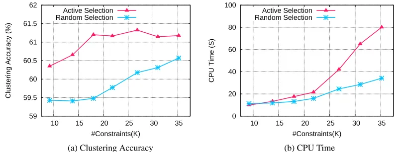
5.3 Active Constraint Selection
To speed up the eigen-decomposition process, instead of engaging all pairwise constraints, we propose to sample a subset of Ti j’s for SimpleNPKL. Instead of acquiring class label information
for kernel learning; here, we consider another simple active constraint selection scheme. Recall that a general principle in active learning is to request the label of the data points that are most uncertain for their predictions. Following this idea, we adopt the margin criterion to measure the uncertainty of the prediction value on a data point. In particular, given a data point xi, assume that we have the
prediction function in the form:
f(xi) =
∑
jyjK(xi,xj).
We can use|yif(xi)|to measure the uncertainty of prediction, where yi∈ {−1,+1}is the class label
of data point xi. As a result, for a data point xi, we choose the constraints involving point i:
i∗ = arg min
i
1
li
∑
jyiyjK(xi,xj)
= arg min
i
1
li j,T
∑
i j6=0
Ti jK(xi,xj)
,
where we deem Ti jas an entry of yy′, and li=|{j :(i,j)∈
S
∪D
},Ti j6=0}|is used as a normalizationof the margin value. Based on the above formula, we choose a subset of k data points
S
k that are most uncertain according to the margin measure. Then, we choose all the Ti j’s that involve any point i∈S
kas pairwise constraints to form a new set of constraints. Finally, we run SimpleNPKL basedon this new set of constraints.
5.4 Low Rank Approximation of K
Since the rank r of K often satisfies r<n, we may express K as K=VEV′, where the columns of Vn×rare eigenvectors of K. If we fix the base V, the number of variables is reduced from n2to r2. With this approximation scheme, the A matrix in Algorithm 1 becomes A=V′(L−∑αi jTi j)V.
Note V′LV can be pre-computed and V′∑αi jTi jV can be computed efficiently by virtue of the
sparseness. Therefore, SimpleNPKL can be significantly faster with this approximation.
6. Applications of SimpleNPKL
In this Section, we extend the proposed SimpleNPKL technique to other similar machine learning problems where the goal of the optimization is to find an optimal matrix such that its inner prod-uct with another matrix is maximized or minimized. In particular, we consider the data embedding problems, where the goal is to find a new data representation that preserves some similarity/distance constraints between pairs of data points. These problems typically can be implemented by con-straining the alignment of the target kernel matrix to some prior affinity or distance structures. As a result, the kernel matrix K=V′V implies a data embedding with a natural interpretation, in which the column vector of V corresponds to the new data representation. We discuss several important data embedding methods below.
6.1 Colored Maximum Variance Unfolding
maximiz-ing the trace of a matrix K subject to some positive definiteness, centermaximiz-ing and distance-preservmaximiz-ing constraints, that is:
minK −tr K : K0,
∑
i j
Ki j=0,tr KTi j=Di j,∀(i,j)∈
N
.where tr KTi j=Kii+Kj j−2Ki j is the square distance between xiand xj.
CMVU interprets MVU from a statistical perspective. It maximizes the dependence between the domain of input pattern x and the domain of label y, which is measured by the Hilbert- Schmidt
Independence Criterion (Gretton et al., 2005; Song et al., 2008). Here we introduce slack
vari-ablesξto measure the violations of distance constraints and penalize the corresponding square loss. Consequently the optimization task of colored MVU is reformulated as:
minK,ξ −tr HKHY+
C
2
∑
ξ 2i j, : K0,tr KTi j=Di j−ξi j,∀(i,j)∈
N
where Hi j=δi j−N−1such that HKH centers K, Y=yy′is the kernel matrix over labels.
Appar-ently this belongs to an SDP problem.
Following the SimpleNPKL algorithms, we derive the minimax optimization problem by intro-ducing dual variables for the inequality constraints:
maxαminK tr
−HYH−
∑
i j αi jTi j
K+
∑
i jαi jDi j−
1 2C
∑
i j α2
i j : K0,tr KK≤B.
(31)
By substituting the following results
A=HYH+
∑
i jαi jTi j and ∇Ji jt =Di j−tr Ti jK−
1
Cα t i j
back into Algorithm 1, the problem of (31) can be solved immediately.
6.2 Minimum Volume Embedding
Minimum Volume Embedding (MVE) is another improvement of MVU (Shaw and Jebara, 2007). One limitation of MVU is that it simply maximizes the trace of K, which may result in the solution that engages considerably more dimensions than necessity. To address this problem, Shaw and Jebara (2007) proposed to grow the top few eigenvalues of K while shrinking the remaining ones. In particular, let K=∑iλiviv′i,λ1≥, . . . ,≥λn, and K0=∑di=1viv′i−∑ni=d+1viv′i. When the intrinsic
dimensionality d is available, MVE formulates the data embedding problem as follows:
To speed up the solution, following the similar derivation in the above CMVU, we can solve (32) by eigen-decomposition in an iterative manner. Specifically, we make the following modifications:
A=K0+
∑
i j
αi jTi j and ∇Ji jt =Di j−tr Ti jK−
1
Cα t i j
By substitute the above results back into Algorithm 1, we can solve the MVE problem efficiently.
6.3 Structure Preserving Embedding
Structure Preserving Embedding (SPE) (Shaw and Jebara, 2009) is a machine learning technique that embeds graphs in low-dimensional Euclidean space such that the embedding preserves the global topological properties of the input graph. Suppose we have a connectivity matrix W, where
Wi j =1 if xi and xj are connected and Wi j =0 otherwise. SPE learns a kernel matrix K such that
the similarity tr KW is maximized while the global topological properties of the input graph are preserved. More formally, the SPE problem is formulated into the following SDP optimization:
minK −tr KW+Cξ : Di j>(1−Wi j)max
m (WimDim)−ξ, ξ≥0
where Di j=Kii+Kj j−2Ki j=tr KTi j is the squared distance between xi and xj.
Let [n] ={1, . . . ,n} and
N
i denote the set of indices of points which are among the nearest neighbors of xi. Then for each point xi, SPE essentially generates(n− |N
i|)× |N
i|constraints:tr KTi j>tr KTik−ξ, ∀i∈[n],j∈[n]−
N
i,k∈N
i.In order to speed up the SPE algorithm, we apply the SimpleNPKL technique to turn the SPE optimization into the following minimax optimization problem:
maxαminK tr
∑
i k∑
∈Ni∑
j∈/Niαi jk(Tik−Ti j)−W
K : K0,tr KK≤B,
∑
αi jk∈[0,C].Similarly, we can derive the following results:
A=W−
∑
i jk
αi jk(Tik−Ti j) and ∇Ji jkt =tr K(Tik−Ti j).
Substituting them back into Algorithm 1 leads to an efficient solution for the SPE problem.
7. Experiments
In this Section, we conduct extensive experiments to examine the efficacy and efficiency of the proposed SimpleNPKL algorithms.
7.1 Experimental Setup
proposed SimpleNPKL algorithms with the NPKL method in Hoi et al. (2007) for kernel k-means clustering. The results of k-means clustering and constrained k-means clustering using Euclidean metric are also reported as the performance of the baseline methods. The abbreviations of different approaches are described as follows:
• k-means: k-means clustering using Euclidean metric;
• ck-means: The constrained k-means clustering algorithm using Euclidean metric and side information;
• SimpleNPKL+LL: The proposed SimpleNPKL with linear loss defined in (12);
• SimpleNPKL+SHL: The proposed SimpleNPKL with squared hinge loss defined in (21); • NPKL+LL: NPKL in (10) using linear loss;
• NPKL+HL: NPKL in (10) using hinge loss.
To construct the graph Laplacian matrix L in NPKL, we adopt the cover tree data structure.2 The sparse eigen-decomposition used in SimpleNPKL is implemented by the popular Arpack toolkit.3 We also adopt the standard SDP solver, SDPT3,4as the baseline solution for NPKL. The pair-wise constraint is assigned for randomly generated pairs of points according to their ground truth labels. The number of constraints is controlled by the resulted amount of connected components as defined in previous studies (Xing et al., 2003; Hoi et al., 2007). Note that typically the larger the number of constraints, the smaller the number of connected components.
Several parameters are involved in both NPKL and SimpleNPKL. Their notation and settings are given as follows:
• k : The number of nearest neighbors for constructing the graph Laplacian matrix L, we set it
to 5 for small data sets in Table 1, and 50 for Adult database in Table 6;
• r : The ratio of the number of connected components compared with the data set size N. In
our experiments, we set r≈70%N which follows the setting of Hoi et al. (2007);
• B : The parameter that controls the capacity of the learned kernel in (11). We fix B=N for
the adult data sets and fix B=1 for the data sets in Table 1 and;
• C : The regularization parameter for the loss term in NPKL and SimpleNPKL. We fix C=1 for the adult data sets and several constant values in the range (0, 1] for the data sets in Table 1.
In our experiments, all clustering results were obtained by averaging the results from 20 different random repetitions. All experiments were conducted on a 32bit Windows PC with 3.4GHz CPU and 3GB RAM.
7.2 Comparisons on Benchmark Data Sets
To evaluate the clustering performance, we adopt the clustering accuracy used in Hoi et al. (2007):
Cluster Accuracy=
∑
i>j1{ci=cj}=1{cˆi=cˆj}
0.5n(n−1) .
2. The cover tree data structure is described athttp://hunch.net/˜jl/projects/cover_tree/cover_tree.html.
3. The Arpack toolkit can be found athttp://www.caam.rice.edu/software/ARPACK/.
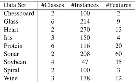
Data Set #Classes #Instances #Features
Chessboard 2 100 2
Glass 6 214 9
Heart 2 270 13
Iris 3 150 4
Protein 6 116 20
Sonar 2 208 60
Soybean 4 47 35
Spiral 2 100 3
Wine 3 178 12
Table 1: The statistics of the data sets used in our experiments.
This metric measures the percentage of data pairs that are correctly clustered together. We compare the proposed SimpleNPKL algorithms with NPKL on the nine data sets from UCI machine learning repositories,5 as summarized in Table 1. The same data sets were also adopted in the NPKL study of Hoi et al. (2007).
The clustering accuracy and CPU time cost (the clustering time was excluded) of different NPKL methods are reported in Table 2 and 3. As can be observed from Table 2, all NPKL meth-ods outperform the baseline k-means clustering and the constrained k-means clustering methmeth-ods, which use Euclidean metric for k-means clustering. The proposed SimpleNPKL with square hinge loss produces very competitive clustering performance to the results of NPKL with hinge loss (as reported in Hoi et al., 2007). SimpleNPKL with square hinge loss and NPKL with hinge loss often perform better than the NPKL methods using linear loss.
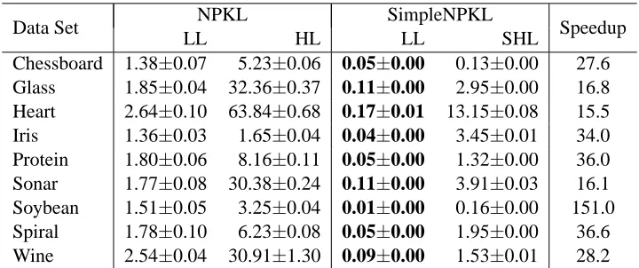
For the CPU time cost, the time costs of SimpleNPKL and NPKL using linear loss are usually lower than those of their counterparts with (square) hinge loss. Regarding the efficiency evaluation in Table 3, our SimpleNPKL with linear loss or squared hinge loss is about 5 to 10 times faster than NPKL using the SDPT3 solver. For some cases of linear loss, SimpleNPKL can be even 100 times faster.
Recall that our key Proposition 1 provides a closed-form solution to the learned kernel matrix K for p≥1, in which the capacity parameter B can be omitted for SimpleNPKL+linear loss. To show the influence of the capacity parameter B for SimpleNPKL + square hinge loss, we present some results in Table 4 with a fixed p=2. To clearly show the influence on convergence, we present the number of iterations instead of elapsed CPU time. We observe that SimpleNPKL + square hinge loss is not sensitive to B on the both Iris and Protein data sets. It even produces the identical accuracy on the Iris data set for B∈ {2.5,3,3.5,4}. However, it affects the number of steps it takes to converge. Similar phenomena can be observed on other data sets.
We also study the clustering performance of varying p in Table 5. We fixed B=1 in this ex-periment. From Table 5, we can observe that SimpleNPKL+square hinge loss produces the best clustering accuracy for the Iris data set when p=4, but the improvement is not significant com-paring with p=2. For the Protein data set, our algorithm achieves the best results when p=2. In general, when p<2, the clustering performance drops significantly.
Data Set k-means ck-means NPKL SimpleNPKL
LL HL LL SHL
Chessboard 49.8±0.2 50.1±0.3 61.1±6.9 56.3±6.1 60.2±0.0 58.8±0.8 Glass 69.7±1.9 69.2±1.7 74.4±3.7 79.1±4.9 73.0±2.5 73.5±2.9 Heart 51.5±0.1 52.3±3.7 86.0±0.3 86.2±0.0 86.8±0.0 89.4±0.1 Iris 84.5±6.5 89.4±8.5 96.0±6.1 97.4±0.0 97.4±0.0 97.4±0.0 Protein 76.2±2.0 80.7±3.1 78.2±3.2 86.4±3.8 81.8±1.8 75.9±2.0 Sonar 50.2±0.1 50.8±0.2 76.8±0.3 64.5±6.8 70.2±10 78.0±0.0 Soybean 82.1±6.1 83.8±8.3 90.2±7.7 100.0±0.0 95.3±5.1 95.4±4.9 Spiral 50.1±0.6 50.6±1.3 86.5±0.0 94.1±0.0 92.2±0.0 94.1±0.0 Wine 71.2±1.2 76.1±2.8 78.1±1.7 85.5±5.3 83.7±4.8 85.0±2.6
Table 2: Clustering accuracy of SimpleNPKL, compared with the results of NPKL in (10) using a standard SDP solver, and k-means.
Data Set NPKL SimpleNPKL Speedup
LL HL LL SHL
Chessboard 1.38±0.07 5.23±0.06 0.05±0.00 0.13±0.00 27.6 Glass 1.85±0.04 32.36±0.37 0.11±0.00 2.95±0.00 16.8 Heart 2.64±0.10 63.84±0.68 0.17±0.01 13.15±0.08 15.5 Iris 1.36±0.03 1.65±0.04 0.04±0.00 3.45±0.01 34.0 Protein 1.80±0.06 8.16±0.11 0.05±0.00 1.32±0.00 36.0 Sonar 1.77±0.08 30.38±0.24 0.11±0.00 3.91±0.03 16.1 Soybean 1.51±0.05 3.25±0.04 0.01±0.00 0.16±0.00 151.0 Spiral 1.78±0.10 6.23±0.08 0.05±0.00 1.95±0.00 36.6 Wine 2.54±0.04 30.91±1.30 0.09±0.00 1.53±0.01 28.2
Table 3: CPU time of SimpleNPKL, compared with the results of NPKL in (10) using a standard SDP solver. (The best results are in bold and the last “Speedup” column is listed only for the linear loss case.)
7.3 Scalability Study on Adult Data Set
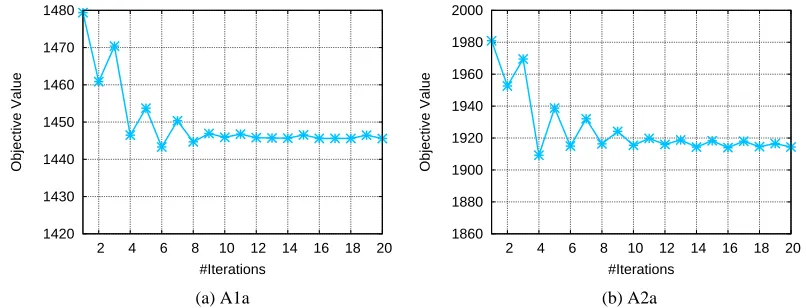
In this Section, we evaluate our SimpleNPKL algorithms on another larger data set to examine the efficiency and scalability. We adopt the Adult database, which is available at the website of LibSVM.6 The database has a series of partitions: A1a, A2a, ···, A5a (see Table 6). Since the training time complexity of NPKL using standard SDP solvers is O(N6.5), which cannot be applied on this database for comparison. We only report the results of both means and constrained k-means clustering as the baseline comparison.
Table 7 shows the clustering performance and CPU time cost (the clustering time was excluded) of SimpleNPKL on the Adult database. From the results, we can draw several observations. First of all, we can see that by learning better kernels from pairwise constraints, both SimpleNPKL al-gorithms produce better clustering performance than that of k-means clustering and constrained