Using Markov Blankets for Causal Structure Learning

(1)

Using Markov Blankets for Causal Structure Learning

Jean-Philippe Pellet∗ [email protected]

Data Analytics Group

IBM Zurich Research Laboratory S¨aumerstraße 4, CH–8803 R ¨uschlikon

Editor: David Maxwell Chickering

Abstract

We show how a generic feature-selection algorithm returning strongly relevant variables can be turned into a causal structure-learning algorithm. We prove this under the Faithfulness assump-tion for the data distribuassump-tion. In a causal graph, the strongly relevant variables for a node X are its parents, children, and children’s parents (or spouses), also known as the Markov blanket of X . Identifying the spouses leads to the detection of the V-structure patterns and thus to causal orien-tations. Repeating the task for all variables yields a valid partially oriented causal graph. We first show an efficient way to identify the spouse links. We then perform several experiments in the con-tinuous domain using the Recursive Feature Elimination feature-selection algorithm with Support Vector Regression and empirically verify the intuition of this direct (but computationally expen-sive) approach. Within the same framework, we then devise a fast and consistent algorithm, Total Conditioning (TC), and a variant, TCbw, with an explicit backward feature-selection heuristics,

for Gaussian data. After running a series of comparative experiments on five artificial networks, we argue that Markov blanket algorithms such as TC/TCbwor Grow-Shrink scale better than the

reference PC algorithm and provides higher structural accuracy.

Keywords: causal structure learning, feature selection, Markov blanket, partial correlation,

statis-tical test of conditional independence

1. Introduction

In this paper, we are interested in using concepts from the feature-selection field to help causal structure learning. Causal structure learning (Pearl, 2000; Spirtes et al., 2001) is a multivariate data-analysis approach that aims to build a directed acyclic graph (DAG) showing direct causal relations among the variables of interest of a given system. These so-called causal graphs can be used together with dedicated rules called do-calculus (Pearl, 1995) to predict the effect of interventions, that is, of structural changes in the data-generating process. In this sense, it differs significantly from traditional machine-learning techniques: given a set of interventions, we can predict the behavior of a set of variables whose joint probability distribution has changed since the model was trained.

Building the causal graph is a difficult task, subject to a series of assumptions, and provably correct algorithms have an exponential worst-case complexity. Identifying the exact causal graph is in general impossible. By means of non-interventional data, causal graphs can only be identified up to observational equivalence: only adjacencies and so-called V-structures (two independent causes

(2)

leading to the same effect) can be specified exactly (Pearl, 2000, p. 19). Typical structure-learning algorithms thus return partially directed acyclic graphs (PDAGs). These algorithms can be roughly classified into two categories: the score-based algorithms associate a score function with a DAG or PDAG given a training data set and perform, for instance, a greedy search in the space of DAGs or PDAGs (e.g., the GES algorithm, Chickering, 2002); the constraint-based algorithms look for dependencies and conditional dependencies in the data and build the causal graph accordingly. Well-known examples are the PC (Spirtes et al., 2001) or the IC (Pearl and Verma, 1991) algorithms. In an effort to get the best of both worlds, other algorithms use both conditional-independence tests and scores to build the network; MMHC (Tsamardinos et al., 2006) is such an example.

The range of data sets that the typical algorithms can deal with is restricted: not any probability distribution can be faithfully represented by a DAG. Faithfulness of the distribution is a well-defined condition: it guarantees the existence of a DAG, called a perfect map, where there is a one-to-one mapping between the graphical criterion of d-separation and conditional independence in the data.1 Nilsson et al. (2007) discuss faithful distributions and other types of distributions with respect to properties of conditional independence. In the literature, Faithfulness is a precondition to prove correctness of the algorithms.

In practice, both existing score-based and constraint-based techniques deal primarily with dis-crete data sets. Score-based approaches for continuous variables are computationally expensive;2 as for the constraint-based approaches, only the multivariate Gaussian case has been dealt with ef-ficiently (Scheines et al., 1995). Margaritis (2005) proposed a distribution-free test of conditional independence, which is very computationally expensive and cannot be readily used with the current constraint-based algorithms for all but very small networks.

Coming from the machine-learning community, feature selection (John et al., 1994; Guyon and Elisseeff, 2003) is a common technique that aims at reducing the number of variables or features used for building more efficient or more robust models. Techniques have evolved to be able to han-dle nonlinear relationships between variables, redundant variables, in both discrete and continuous domains. Feature selection and causal structure learning are related by a common concept: the

Markov blanket of a variable X is the smallest set Mb(X)containing all variables carrying informa-tion about X that cannot be obtained from any other variable.3 In feature selection, this is the set of

strongly relevant features; that is, of features which carry information about the target that cannot

be obtained from any other variable (Kohavi and John, 1997). In a causal graph, this is the set of all parents, children, and spouses of X . The feature-selection task and the causal graph construction task can both be stated to some extent as Markov blanket identification tasks.

Relating feature selection and causal structure learning is not new. Several algorithms identify-ing the Markov blanket of a sidentify-ingle variable with techniques inspired from causal structure learnidentify-ing have been proposed as the optimal solution to the feature-selection problem in the case of a faithful distribution. Tsamardinos and Aliferis (2003) show that for faithful distributions, the Markov blan-ket of a variable Y is exactly the set of strongly relevant features, and prove its uniqueness. They propose the Incremental Association Markov Blanket (IAMB) algorithm to determine it. With the same Faithfulness assumption, the Min-Max Markov Blanket algorithm (MMMB) (Tsamardinos

1. Conditional independence and d-separation are defined formally in Section 2.

2. Computationally tractable methods to learn Bayesian networks from continuous data exist (Fu, 2005), like Bach and Jordan (2003), but do not offer the causality-related theoretical correctness guarantees.

(3)

et al., 2003) identifies the Markov blanket of a variable Y by calling a subroutine Min-Max Parents and Children (MMPC). This subroutine finds the direct parents and children of Y with associa-tion measures and condiassocia-tional-independence tests. MMPC is again called on each of these nodes to find potential spouses of Y . False positives are then discarded with conditional-independence tests. MMMB was further discussed by Pe ˜na et al. (2005), who propose AlgorithmMB, a similar approach based on scores and conditional-independence tests to retrieve Mb(Y). The HITON MB algorithm (Aliferis et al., 2003) is similar in its main steps, and selects an optimal subset of the Markov blanket of a target variable given the Faithfulness assumption. Nilsson et al. (2007) also propose a theoretical algorithm for consistent identification of strongly relevant features in poly-nomial time for the class of strictly positive distributions. They also argue that some common backward feature-elimination algorithms like Recursive Feature Elimination (Guyon et al., 2002) are actually consistent, in the sense that they return the set of strongly relevant features in the large sample limit.4

These are examples of using causal structure learning or similar constraint-based techniques to help feature selection (see Guyon et al., 2007, for a review of those techniques). In this paper, we propose a framework to do the converse. We present a generic approach using the outcome of a consistent feature-selection algorithm FS to build an approximate structure of the true causal graph. If we assume that FS returns the Markov blanket of the variables, we can show how to turn this approximate result, called moral graph (Lauritzen and Spiegelhalter, 1988), into a provably correct PDAG depicting the causal structure. This approach is also used in the Grow-Shrink algorithm (Margaritis and Thrun, 1999), which also builds a moral graph before adjusting the local structure.

This paper contributes a generic algorithm to build a causal graph which clearly separates the Markov blanket identification and the needed local adjustments, an efficient algorithm to perform those adjustments, and two fast instances of the generic algorithm for multivariate Gaussian data sets. This is presented as follows: in Section 2, we first review the needed terms and definitions from feature selection and causality. In Section 3, we make the link from the outcome of a feature-selection algorithm to a causal graph by detailing the needed local adjustments and detail an efficient way to perform them. We directly apply it in Section 4, where we describe how we can build causal graphs using the RFE feature-selection algorithm. As this direct application is very computationally intensive, we then show our more efficient instantiations of the generic algorithm optimized for the multivariate Gaussian case, the TC and TCbwalgorithms. We list our experimental results in Section 5, showing through empirical evaluation that Markov blanket algorithms are more scalable and more accurate than the reference PC algorithm. We finally conclude in Section 6 and list proofs in Appendix A.

1.1 Notation

Boldface capitals designate either matrices or sets of random variables or nodes in a graph, depend-ing on the context. V is the set of all variables in the analysis. Italicized capitals like X,Y,Z are

random variables or nodes and elements of V. Vectors are set in boldface lowercase, as b or w; scalars in italics, as the number of samples n or the number of variables (the problem dimension) d. We indiscriminately write “variable” or “feature” to refer to any variable in the causal analysis or

(4)

any node in a causal graph, and write “predictor” to designate a variable used as input for a given classifier or regression model.

2. Background

We formalize the feature-selection task suited for our needs and provide relevant definitions. We do the same for the causal structure-learning task and prepare the needed basis for drawing the parallels between the two in the next section.

2.1 Feature Selection

We are given a data set of n samples D={(xi,yi),1≤i≤n}. Each data point(xi,yi) has d−1 inputs, modeled as a vector xi∈Rd−1, and an output, or target, yi∈R(we use d−1 and not d for

the size of xi for consistency with the rest of the paper). The data points are assumed to be drawn

i.i.d. from a joint probability distribution over the random variables V=X∪ {Y}. The result of the feature-selection task we are interested in is a set of retained variables F⊆X. How many variables to retain and which variables to retain depends on the particular algorithm, and usually maximizes some tradeoff between efficiency and classification/regression error of a given learning task.

John et al. (1994) propose a classification of the input variables X with respect to their relevance to the target Y in terms of conditional independence.

Definition 1 (Conditional independence) In a variable set V, two random variables X,Y are

con-ditionally independent given Z⊆V\ {X,Y}, noted(X⊥⊥Y |Z), if: ∀x,y,z : P(X=x|Y =y,Z=z) =P(X=x|Z=z), provided that∀z : P(Z=z)>0.

Conditional independence is a generalization of the traditional notion of statistical independence. If two variables X and Y are independent, then the joint distribution is the product of the marginals:

P(X=x,Y=y) =P(X=x)P(Y=y). If they are dependent given some conditioning set Z, then we can write P(X=x,Y =y|Z=z) =P(X=x|Z=z)P(Y=y|Z=z). Conditional independence is a key concept in Bayesian networks (Pearl, 1988) because of the factorizations of the joint probability distribution it allows.

In feature selection, relevance of predictors to the target as proposed by John et al. (1994) is expressed in terms of conditional independence. In the following definitions, we write Xi to note

the ith input variable, and X\ito note all input variables but the ith one.

Definition 2 (Strong relevance) A variable Xiis strongly relevant to the target Y if P(Y|X\i)6=P(Y|X\i,Xi).

A variable is strongly relevant to the target if it carries information about Y that no other variable carries. This is expressed in the definition by a change in the probability distribution of the target between conditioning on all other variables, X\i, and also including Xi in the conditioning set. If Xi

(5)

Definition 3 (Weak relevance) A variable Xiis weakly relevant to the target Y if it is not strongly relevant and

∃S⊆X_\i: P(Y|S)6=P(Y|S,Xi).

We speak of weak relevance of a variable Xiwhen there exists a certain context S in which it carries

information about the target. However, this is not necessarily exclusive information, as it may be possible to obtain it from other variables.

Corollary 4 (Irrelevance) A variable Xi is irrelevant to the target Y if it is neither strongly nor weakly relevant, that is, if

∀S⊆X_\_i: P(Y|S) =P(Y|S,Xi).

A variable is irrelevant if carries no information about the target at all, no matter what the context is.

For our purposes, we assume that the feature-selection algorithm returns the set of all strongly relevant variables, and only those.5 (In Section 5, we discuss with experiments whether this is a reasonable assumption with the RFE algorithm.) Put in terms of conditional independence, the result FY of the feature-selection task with target Y is, with V=X∪ {Y}:

FY =

X (X6⊥⊥Y |V\ {X,Y}) . (1)

That is the set of the variables that are dependent on the target Y , conditioned on all others. We need this property in Section 3 to use the output of the feature-selection task to build a causal graph. Note that if we repeat the feature-selection task using as target another variable X ∈V yielding a result FX, we have:

X∈FY ⇐⇒ Y ∈FX. (2)

This follows as a direct consequence of (1) due to the symmetry of the conditional-independence relation(X ⊥⊥Y |Z)with respect to X and Y .

2.2 Causal Structure Learning

In causal structure learning, we are interested in representing graphically conditional dependencies found in the data. Under a set of assumptions, they have a causal interpretation. For this task, we have a data set of n samples D={vi,1≤i≤n}. We do not designate a specific target variable in V as we are interested in learning the full structure of the network.

The graphical representation of choice for causal models is directed acyclic graphs (DAGs) (Pearl, 2000). In a causal graph represented by a DAG, we want to represent direct causal relations with arcs between pairs of variables. Choosing DAGs for this task implies restrictions, an obvious one of which is that causal feedback loops are excluded from the analysis. More formally, the joint probability distribution has to be faithful (or DAG-isomorphic, Pearl, 1988, p. 128); that is, there must exist a DAG that represents all (conditional) dependencies and independencies entailed by the distribution. Such a graph is called a perfect map of the distribution if there is a one-to-one mapping between the conditional-independence relation defined on variables and the d-separation criterion defined on the graphical nodes.

(6)

Definition 5 (d-separation) In a DAG

G

, two nodes X,Y are d-separated by Z⊆V\{X,Y}, written (X ↔| Y |Z), if every path from X to Y is blocked by Z. A path is blocked if at least one diverging or serially connected node is in Z or if at least one converging node and all its descendants are not in Z. If X and Y are not d-separated by Z, they are d-connected:(X ↔Y |Z).

Determining whether two nodes in a graph are d-separated given some conditioning set is not visually immediate. It may for instance be unintuitive that whereas conditioning on a node W on a directed path X →W →Y blocks the path from X to Y , conditioning on a common child Z of

two variables X,Y in X →Z←Y connects them. In the latter case, this common child is called a collider. If, furthermore, two parents X,Y of a node Z are nonadjacent in the full graph, then Z is

called an unshielded collider for the pair(X,Y).

The definition of d-separation was worked out by Pearl (1988) to match as closely as possible the complicated nature of the conditional-independence relation with a graphical criterion, so that the class of faithful distributions, which can be represented by a perfect map, is as large as possible, while still keeping a natural graphical representation.

Definition 6 (Perfect map) A DAG

G

is a directed perfect map of a joint probability distribution P(V)if there is bijection between d-separation in

G

and conditional independence in P:

∀X,Y ∈V,∀Z⊆V\ {X,Y}: (X ↔| Y |Z) ⇐⇒ (X⊥⊥Y |Z)

. (3)

If we take apart the perfect-map equivalence, we distinguish two important concepts, known as the Causal Markov condition and the Faithfulness condition (Spirtes et al., 2001, p. 29).

The Causal Markov condition is said to hold for a graph

G

=hV,Eiand a probability distribu-tion P(V)if every variable is statistically independent of its graphical non-descendants (intuitively, of its non-effects, direct or indirect) conditional on its graphical parents (intuitively, its direct causes) in P. Pairsh

G

,Pithat satisfy the Causal Markov condition satisfy the implication

∀X,Y ∈V,∀Z⊆V\ {X,Y}: (X↔| Y |Z) =⇒ (X⊥⊥Y |Z)

.

This is called I-map property by Pearl (1988).

The Faithfulness condition can be interpreted as the converse of the Causal Markov condition, and states that the only conditional independencies to hold are those specified by the Causal Markov condition:

∀X,Y ∈V,∀Z⊆V\ {X,Y}: (X↔Y |Z) =⇒ (X6⊥⊥Y |Z)

.

If the Causal Markov and Faithfulness conditions hold together for a pairh

G

,Pi, then we find again the equivalence (3), and

G

is a perfect map of P.

(7)

unconditionally independent of every other, but any variable pair becomes dependent conditioned on all other variables. On this problem, current constraint-based algorithms yield an empty graph because of the pairwise unconditional independencies, although it is not true that the data shows no dependency at all since one variable is a well-defined function of all others.

From this point on and for all proofs, we assume that the working data set D has a distribution that does not violate Faithfulness, and that it can thus be represented by a perfect map. In such a context, however, it is still not clear that causation can be inferred from conditional independence. We now proceed to explain the relation between causation and conditional independence.

Assuming Faithfulness, direct causation between X and Y , noted X_{_}Y , implies that X and Y

are dependent given any conditioning set (Pearl and Verma, 1991, see definitions of potential and genuine causes):

X_{_}Y =⇒ ∀S⊆V\ {X,Y}:(X6⊥⊥Y |S) .

We denote the absence of direct causation by X 6_{_}Y . The exact converse of this implication does

not hold. If we make the Causal Sufficiency assumption (Spirtes et al., 2001), that is, assume that no hidden common cause of two variables exists, we can write:

∀S⊆V\ {X,Y}:(X6⊥⊥Y |S)

=⇒ X_{_}Y or Y _{_}X. (4)

Using (4), we can theoretically determine all adjacencies of the causal graph with conditional-independence tests, but we cannot orient the edges. But there is a special causation pattern where conditional-independence tests can reveal the direction of causation. It is known as a V-structure (Pearl, 2000): two common causes X,Y , initially independent,6 become dependent when condi-tioned on a common effect Z, then acting as a collider. This is noted X _Z^Y , where we also require X 6_{_}Y and, symmetrically, Y6_{_}X . Formally, we have:

X _{_}Z_^Y and X6_{_}Y and Y 6_{_}X

=⇒ ∃S⊆V\ {X,Y,Z}:(X ⊥⊥Y |S) and(X6⊥⊥Y |S∪ {Z})

.

The exact converse does not hold either. But using (4), we can find an equivalence relation defining a V-structure, still assuming Causal Sufficiency: first, we certify the existence of a link between

X and Z and between Y and Z. Z is then identified as an unshielded collider if conditioning on it

creates a dependency between X and Y :

X_Z^Y ⇐⇒

∃S⊆V\ {X,Y,Z}:(X ⊥⊥Y |S) and(X6⊥⊥Y |S∪ {Z})

and ∀S⊆V\ {X,Z}:(X6⊥⊥Z |S)

and ∀S⊆V\ {Y,Z}:(Y 6⊥⊥Z |S)

. (5)

Actually, typical algorithms first establish the existence of a link between two variables by seeking a certificate equivalent to, or implicating the premise of, (4), and then look for orientation possi-bilities. Note that there is no guarantee that all links can be oriented into causal arcs, and that in

(8)

general we therefore cannot recover the full causal structure with conditional-independence tests. This is the problem known as causal underdetermination (Spirtes et al., 2001, p. 62): for the structure-learning task given observational data, a correct graph is specified by its adjacencies and its V-structures only. Partially oriented graphs returned by structure-learning algorithms represent

observationally equivalent classes of causal graphs (Pearl, 2000, p. 19). This means that for a given

joint probability distribution P(V), the set of all conditional-independence statements that hold in P does not yield a unique perfect map in general.

Formally, if we combine (3), (4) and (5), we find, for a perfect causal map

G

(using the symbol “_{_}” to denote direct causation and “→” to denote an arc in the graph):

X,Y adjacent in

G

⇐⇒ X_{_}Y or Y _{_}X

X→Z←Y ⇐⇒ X_{_}Z_^Y. (6)

It is sometimes possible to orient further arcs in a graph by looking at already-oriented arcs and propagating constraints, preventing acyclicity and the creation of additional V-structures other than those already detected. The graph after this constraint-propagation step is called completed PDAG,

maximally oriented PDAG (CPDAG), or essential graph, depending on the author.

3. Causal Network Construction Based on Feature Selection

We have looked at the ideal outcome of feature selection in (1) and how to read a causal graph in (6). We now turn to showing how feature selection can be used to build a causal graph. From now on and for the rest of this paper, we assume that the joint probability distribution over all variables V is faithful.

3.1 Identifying the Markov Blankets

In the context of directed graphical models, the Markov blanket of a node X , noted Mb(X), is the set of parents, children, and children’s parents (spouses) of X . As an easy property, note that we have:

X∈Mb(Y) ⇐⇒ Y ∈Mb(X).

The following statement is a key property of Markov blankets.

Property 7 (Total conditioning) In the context of a faithful causal graph

G

, we have:

∀X,Y ∈V : X∈Mb(Y) ⇐⇒ (X6⊥⊥Y |V\ {X,Y})

.

(See Appendix A for the proof.) This property says that the Markov blanket of each node is the set of all variables that are dependent on it, conditioned on all other variables. In other words, in a causal graph, the parents, children, and spouses of Y store information about Y that cannot be obtained from any other variable. Note that Mb(Y) then has exactly the property of the output of feature selection, FY, as characterized in (1). This links feature selection and causal structure

learning in the sense that

(9)

the Faithfulness assumption guaranteeing the unicity of Mb(Y). However, Markov blankets alone do not fully specify a causal graph. Thus, feature selection, even if guaranteed to find only strongly relevant features, cannot be directly used to construct the graph as we want it to be. The problem is that spouses of Y , even if not directly linked in the original graph, would be linked in FY and

Mb(Y). An additional step is needed to transform the Markov blankets into parents, children, and spouses.

3.2 Recovering the Local Structure

The result of feature selection can be graphically shown by an undirected graph

G

=hV,Eiwhere

(X,Y)∈E⇔X ∈FY. This graph is close to the original causal graph in that it contains all arcs as

undirected links, and additionally links spouses together, and is called the moral graph of the orig-inal directed graph (Lauritzen and Spiegelhalter, 1988, p. 166). The extra step needed to transform this graph into a causal PDAG is the deletion of the spouse links and the orientation of the arcs, a task which we call “resolving the Markov blankets.”

An existing algorithm can resolve the Markov blankets, that is, use Markov blanket information to infer the local structure around a node: the Grow-Shrink (GS) algorithm, proposed by Margaritis and Thrun (1999). The full algorithm first finds the Markov blanket for each variable, and performs further conditional-independence tests around each variable to infer the structure locally. It then uses a heuristics to remove cycles possibly introduced by previous steps. We list in Algorithm 1 (using our notation) the steps of the algorithm responsible for building the local structure using the Markov blanket information, as this is exactly the task we are trying to solve. In the code, Bd(X) stands for the boundary of X ; that is, the set of its direct neighbors in the graph

G

. It is different from Mb(X)in that whereas Mb(X) is passed as input to the algorithm and is fixed, Bd(X)depends on the graph

G

, which is modified throughout the algorithm. We note a conditional-independence test with a subroutine call to CONDINDEP(X,Y,Z): ideally, this function returns true when(X⊥⊥Y |Z) holds, and false otherwise. More will be said about the actual implementation of such tests in Section 4. The command break is used to break out of the innermost loop, saving unnecessary computations.

The GS algorithm makes two passes over all variables and the members of their Markov blankets (or direct neighbors in the second pass). It first removes the possible spouse links between linked variables X and Y by looking for a d-separating set around X and Y . In a second pass, it orients the arcs whenever it finds that conditioning on a middle node creates a dependency. While searching for the appropriate conditioning set, GS selects the smallest base search set (set B in Algorithm 1) for each phase. This has two very desirable effects. First, it reduces the number of tests, which is useful because each phase contains a subset search, exponential in time complexity with respect to the searched set. Second, it reduces the average size of the conditioning set, which increases the power of the statistical tests, and thus helps reduce the number of Type II errors.

While the GS approach considerably reduces the number of tests to be performed with respect to a large subset search, it is possible to perform fewer tests while still identifying correctly the structure and orienting the arcs, and decreasing the average conditioning set size. A helpful obser-vation is that orientation and removal of the spouse links can be done together in a single pass. We know, as discussed in the previous section, that only arcs in V-structures can be oriented: fortu-nately, V-structures are exactly spotted when we identify a spouse link to be removed. Two spouses

(10)

Algorithm 1 Resolve the Markov Blankets with the Grow-Shrink Algorithm 1: procedure RESOLVEMARKOVBLANKETS GROWSHRINK

Input: Mb(·): the Markov blanket information for each node X∈V Output:

G

: partially oriented DAG

/* Compute graph structure */

2:

G

←moral graph according to Mb(·) 3: for each X ∈V and Y ∈Mb(X)do

4: B←smallest set of{Bd(X)\ {Y},Bd(Y)\ {X}}

5: for each S⊆B do

6: if CONDINDEP(X,Y,S)then remove link X−Y from

G

; break

7: end for

8: end for

/* Orient edges */

9: for each X ∈V and Y ∈Bd(X)do 10: for each Z∈Bd(X)\Bd(Y)\ {Y}do

11: orient Y →X /* to be corrected if a test yields independence */

12: B←smallest set of{Mb(Y)\ {Z},Mb(Z)\ {Y}}

13: for each S⊆B do

14: if CONDINDEP(Y,Z,S∪ {X})then remove orientation Y→X ; break

15: end for

16: if Y →X then break

17: end for

18: end for 19: return

G

20: end procedure

nodes. Thus, if we can find a set SXY that makes X and Y conditionally independent, we know that

the link between them is a spouse link to be removed. Moreover, we know that any node Z part of the intersection of their Markov blankets not included in SXY is a collider and thus a common

child, and that the triplet(X,Z,Y)is actually a V-structure X→Z←Y in the original graph. This

follows from the definition of d-separation. What we need is an efficient search algorithm to find such d-separating sets.

An approach based on this observation has two main benefits. First, it only searches the trian-gles, that is, the cliques of three nodes, in the moral graph. Assuming that the information about the Markov blanket is correct, only triangles can hide spouse links and V-structures. Second, for each connected pair X−Y in a triangle, decisions about possible spouse links and arc orientation

are taken together and thus faster.

Pseudocode for the proposed search algorithm is listed in Algorithm 2, where the notation

G

\XY

(11)

Definition 8 (Collider sets) In an undirected graph

G

=hV,Ei, let Tri(X−Y)(with X,Y ∈V and

(X,Y)∈E) be the set of vertices forming a triangle with X and Y : Tri(X−Y) ={Z∈V|(X,Z)∈E,(Y,Z)∈E}.

Suppose that

G

is the moral graph of the DAG representing the causal structure of a faithful data set. A set of vertices Z⊆Tri(X−Y)then has the Collider Set property for the pair(X,Y) if it is the largest set that fulfills

∃SXY ⊆V\ {X,Y} \Z :(X⊥⊥Y |SXY) (7)

and ∀Zi∈Z :(X6⊥⊥Y |SXY∪ {Zi}). (8)

The set SXY is then a d-separating set for X,Y .

Lemma 9 In the context of a faithful causal graph, the set Z that has the Collider Set property for

a given pair(X,Y)exists if and only if X is neither a direct cause nor a direct effect of Y . This set

Z is unique when it exists. (Proof in Appendix A.)

The purpose of Algorithm 2 is thus to find these collider sets (in the pseudocode, the symbol( denotes the strict subset relation). The algorithm loops over all triangle links and performs a collider set search for each of them. Let X−Y be one of these links: if it is not a spouse link, the search

procedure will leave the value of the d-separating set SXY to its default value, null. Otherwise, SXY

will be set to a (possibly empty7) set for X and Y . The collider set can be inferred by removing the d-separating set from the triangle nodes Tri(X−Y): as Tri(X−Y) contains nodes on a path of length 2 between X and Y , finding a d-separating set that does not contain some of these nodes proves that they can only be colliders according to the definition of d-separation.8 For instance, if the procedure produces an empty set for a given linked pair X−Y , then X and Y are unconditionally

independent, and therefore all nodes in Tri(X−Y)are colliders.

Two caveats have to be observed during this search, however. First, there might be other active,

d-connecting paths between X and Y that are not going through any node of Tri(X−Y). Those nodes must be blocked by appropriate conditioning on the boundary of X or Y as determined by the base conditioning set at line 6. Second, this base conditioning set must be checked not to include any descendant of possible colliders. If it did, it would open a d-connecting path according to Definition 5. This check is performed at lines 13 to 21. At line 13, we build a set D that includes all possible descendants of currently conjectured colliders that intersect our base conditioning set B. The following loop makes sure none of them was opening a path between X and Y .

Theorem 10 In the large sample limit, for faithful, causally sufficient data sets, the procedure RE

-SOLVEMARKOVBLANKETS COLLIDERSETS correctly identifies all V-structures and all spouse

links, assuming consistent statistical tests. (Proof in Appendix A.)

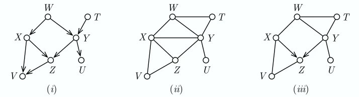
This procedure is best understood with a graphical example. Consider the sample local struc-ture in Figure 1, imagine it is part of a larger network, and suppose we are performing the search

7. Note that returning an empty d-separating set in SXY is different from returning null, signaling the absence of any such set.

(12)

Algorithm 2 Resolve the Markov Blankets with Collider Sets 1: procedure RESOLVEMARKOVBLANKETS COLLIDERSETS

Input: Mb(·): the Markov blanket information for each node X∈V Output:

G

: partially oriented DAG

2:

G

←moral graph according to Mb(·)

3: C← {}, an empty list of orientation directives

4: for each edge X−Y part of a fully connected triangle do

5: SXY ←null /* search for d-separating set */

6: B←smallest set of{Bd(X)\Tri(X−Y)\ {Y},Bd(Y)\Tri(X−Y)\ {X}}

7: for each S(Tri(X−Y)do /* subset search */

8: Z←B∪S

9: if CONDINDEP(X,Y,Z)then

10: SXY ←Z

11: break to line 23

12: end if

13: D←B∩

nodes reachable by W in

G

\XY |W∈ Tri(X−Y)\S

14: B0←B\D

15: for each S0(D do /* descendant of collider may be opening a path */

16: Z←B0∪S0∪S

17: if CONDINDEP(X,Y,Z)then

18: SXY ←Z

19: break to line 23

20: end if

21: end for

22: end for

23: if SXY 6=null then /* save orientation directive */

24: mark link X−Y as spouse link in

G

25: for each Z∈ Tri(X−Y)\SXY

do

26: C←C∪ {(X→Z←Y)}

27: end for

28: end if

29: end for

30: remove all spouse links (i.e., marked links) from

G

31: for each orientation directive(X→Z←Y)∈C do /* orient edges */ 32: if edges X−Z and Y−Z still exist in

G

then

33: orient edges as X →Z←Y

34: end if

(13)

X Y

Z W

U V

T

X Y

Z W

U V

T

X Y

Z W

U V

T

(i) (ii) (iii)

Figure 1: Sample local causal structure(i)and corresponding moral graph(ii). On(iii), the spouse link and orientation information that the collider set search for the linked pair X−Y gives.

starting at line 5 in Algorithm 2. We are looking for a d-separating set for X and Y . Looking at the original graph, we see that {W} is the smallest such set; let us see how the algorithm finds it. We have: Tri(X−Y) ={W,Z}, Bd(X) ={W,Y,Z,V}and Bd(Y) ={W,X,Z,U,T}. The base conditioning set B will thus be the smallest of{V},{U,T} , thus B={V}. At this stage, condi-tioning on V is justifiable: one cannot exclude situations where X and Y are d-connected given the empty set through T and V , for instance if T and V both had a common cause farther away in the network. But actually in this example, all (perfect) tests containing V in the conditioning set will yield dependence, because it is a descendant of the collider Z and thus opens a path by definition of d-separation. Eventually, in the iteration where S={W}, we will find conditional independence in the nested loop at lines 15 to 21. As Tri(X−Y)\S={Z}, D will be assigned the value{V}

and B0will be empty, so that we will perform exactly one extra test at line 17 with the conditioning set SXY ={W}, which yields independence. This in turn allows us to identify the link X−Y as a

spouse link and determine (line 25) that the set Tri(X−Y)\SXY ={Z}is the set of all direct effects

of X and Y ; that is, fulfills the Collider Set property.

X Y

Z W

(i)

X Y

Z W

(ii)

X Y

Z W

(iii)

X Y

Z W

(iv)

Figure 2: Another sample local causal structure(i)and corresponding moral graph(ii). On(iii), a wrong result if orientation is done immediately at line 26 of Algorithm 2. On(iv), the correct (non-)orientation if the condition at line 32 is added.

For some structures, the order in which arcs are removed and oriented must happen such that all spouse links are removed before proceeding to orientation. Consider another example, shown in Figure 2, and suppose again that that we are looking for a d-separating set for the pair(X,Y). As

X and Y are unconditionally independent, SXY =/0is a valid d-separating set. We may thus remove

(14)

X→W←X (leaving the spouse link W−Y to be removed later). This would be wrong, precisely

because W−Y is a spouse link, and thus the orientation X →W ←X is not allowed if one of

the links to be oriented does not actually exist in the original graph. This is the reason why all orientation directives are saved in a list C at line 26 of Algorithm 2. After all spouse links have been removed, the orientations are done at line 33 only when both links to be oriented still exist, thus ensuring the existence of the V-structure X→Z←Y .

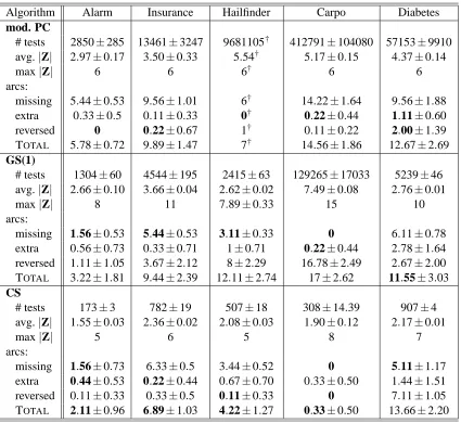
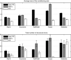
We do not claim that our algorithm uses the smallest possible conditioning set for the tests. There is a tradeoff between obtaining the minimal possible conditioning set and keeping the total number of tests low in the average case. In the empirical evaluation of this algorithm, we examine three behavioral criteria: the total number of tests, the average size of the conditioning set, and the maximum size of the conditioning set.

The complexity of the whole algorithm iterating over all triangle links, in terms of number of calls to CONDINDEP, is

O

(d22α), where d is the number of variables andα=maxX∈V|Mb(X)| −1. In the worst case of a fully connected graph, where Mb(X) =V\ {Y}, it is exponential in the num-ber of variables due to the subset search. But in practice, the original graphs are often sparse enough so that the actual run time is not exponential. Many algorithms (e.g., MMMB, HITON MB, Algo-rithmMB, GS) perform subset searches in the (possibly augmented) Markov blanket and thus rely on graph sparseness to be efficient. Although the complexity of RESOLVEMARKOVBLANKETS

COLLIDERSETSis the same as that of RESOLVEMARKOVBLANKETS GROWSHRINK, we show in

the experimental results in Section 5 that the former performs fewer tests with a smaller average conditioning set size, while still providing comparable accuracy in structure learning.

3.3 A Generic Algorithm Based on Feature Selection

Thanks to the subroutine explained in the previous section, we can now draft a generic algorithm for structure learning based on feature-selection methods returning strongly relevant features. Al-gorithm 3 lists pseudocode for the three main steps of this approach:

1. Find the conjectured Markov blanket of each variable with feature selection and build the moral graph;

2. Remove spouse links and orient V-structures using collider sets; 3. Propagate orientation constraints.

For the sake of completeness, the constraint propagation rules of Step 3 have also been listed, in a separate subroutine (see Algorithm 4). They are common in structure learning to obtain a completed PDAG (Pearl and Verma, 1991). Meek (1995) proves that these three rules indeed return the maximally oriented graph when given a PDAG whose V-structures are oriented.

(15)

Algorithm 3 Causal Structure Learning with Feature Selection 1: procedure GENERICSTRUCTURELEARNING

Input: D : n×d data set with n d-dimensional data points

Output:

G

: maximally oriented partially directed acyclic graph /* Step 1: Markov blanket construction */

2: for each variable X∈V do

3: FX ←FEATURESELECTIONALGORITHM(X,D)

4: end for

5: for each pair(X,Y)such that Y ∈FX and X∈FY do /* symmetry check */

6: add X to Mb(Y)and Y to Mb(X)

7: end for

/* Step 2: Spurious arc removal & V-structure detection */

8:

G

←RESOLVEMARKOVBLANKETS(Mb(·))

/* Step 3: Constraint propagation */

9:

G

←COMPLETEPDAG(

G

)

10: return

G

11: end procedure

Algorithm 4 Orient a PDAG maximally 1: procedure COMPLETEPDAG

Input:

G

: partially directed acyclic graph

Output:

G

: maximally oriented partially directed acyclic graph 2: while

G

is changed by some rule do /* fixed-point iteration */ 3: for each X,Y,Z such that X→Y−Z do

4: orient as X →Y →Z /* no new V-structure */

5: end for

6: for each X,Y such that X−Y and∃directed path from X to Y do

7: orient as X →Y /* preserve acyclicity */

8: end for

9: for each X,Y s.t. X−Y &∃nonadj. Z,W s.t. X−Z→Y & X−W →Y do

10: orient as X →Y /* three-fork V with married parents */

11: end for

(16)

shown to miss strongly relevant variables (Guyon and Elisseeff, 2003). Nilsson et al. (2007) also describe forward selection as inconsistent, but claim that backward feature elimination is actually consistent in the large-sample limit.9 For finite data sets, Statnikov et al. (2006) further show (among others) that even the weights of the irrelevant variables can get bigger than that of relevant variables, and that weakly relevant variables can be selected more often than strongly relevant variables in some cases.

These considerations are taken into account in our approach. In the next section, we describe an instantiation of the generic algorithm with an existing backward feature-elimination algorithm. Expecting the feature selection to be too inclusive, that is, to include features that are not strongly relevant, we add the filtering condition at line 5 of the generic outline in Algorithm 3: in order to link X and Y in the moral graph, we require the feature selection performed for X to have selected variable Y , and conversely, we require X to have been selected by the feature selection performed for Y . This does not theoretically guarantee the absence of “false positives,” however. Further in the section, we replace the feature-selection step with a provably consistent algorithm in the multivariate Gaussian case, and analyze its complexity and behavior.

4. Algorithms for Causal Feature Selection

In this section, we show two algorithms (and a variant) as instantiations of the generic approach previously described. First, we explain an algorithm based on the Recursive Feature Elimination (RFE) algorithm (Guyon et al., 2002) as a direct application of existing methods. We then describe Total Conditioning (TC), a fast algorithm that can be proved correct under the multivariate Gaussian assumption. We also show a variant, TCbw, that improves accuracy with low sample sizes by using an explicit backward feature-selection heuristics. In Section 5, we report on experiments including these algorithms.

4.1 An RFE-Based Approach

To empirically test the soundness of the approach, we propose to use RFE over a Support Vector Regression (SVR) learner (Smola and Sch ¨olkopf, 1998) with a linear kernel, assuming for this example that we will deal with multivariate Gaussian data. RFE is an instance of a backward feature-elimination algorithm. Given some learner (in this case, SVR), it iteratively trains it, ranks the features according to some criterion, and remove the feature (or the p features) with the smallest ranking criterion. This criterion can be the weights w attributed to the features by the learner, or some sensitivity measure of the features (Guyon et al., 2002). In our case, we used the weights w of SVR as described in Smola and Sch ¨olkopf (1998).

Using RFE, the Markov blanket identification is done in two steps:

1. Use RFE to rank the predictors according to their weights in the trained model and to provide what can be seen as a relevance ordering of the predictors;

2. Determine the size of the Markov blanket and thus the number of variables to select from the list returned by RFE.

(17)

We do not have a theoretical guarantee that RFE/SVR will return the Markov blanket variables. Although Nilsson et al. (2007) shows that RFE/SVM as described in Guyon et al. (2002) is con-sistent (i.e., returns strongly relevant variables in the large-sample limit), the limitations of ranking variables on the w weights of an SVM with finite data sets have also been highlighted (Hardin et al., 2004; Statnikov et al., 2006). For now, we thus use this feature-selection step as a heuristics.

In order to determine the number of variables to select from the ranked list returned by RFE, we use the following criterion: starting with the first variable from the list, accept a new variable in the Markov blanket if the cross-validated training error of the SVR decreases with the new variable, and stop and return the current list if adding the next variable increases the error.

Algorithm 5 An RFE-Based Feature-Selection Step 1: procedure RFEFEATURESELECTION

Input: X : the target variable to perform feature selection for

D : n×d data set with n d-dimensional data points

Output: S : the set of selected variables

2: w←weights of V\X according to RFE(SVR)

3: P←predictor variables sorted according to w

4: S← /0

5: erroropt←var[X] /* MSE of constant function */ 6: error←TRAIN(cross-validated SVR with predictor(P)1)) 7: while error<erroropt do

8: erroropt ←error

9: S←S∪ {(P)1} /* add beneficial predictor */

10: P←P\ {(P)1}

11: error←TRAIN(cross-validated SVR with predictors S∪ {(P)1}) 12: end while

13: return S 14: end procedure

The symmetry condition (2), X ∈FY ⇔Y ∈FX, might not be satisfied: we rely on the check at

line 5 of the generic approach of Algorithm 3 to make sure that we do not select spurious features in the Markov blanket. This conservative approach implies that we expect RFE to select at least all strongly relevant variables, plus possibly some others that we hope to identify with this simple condition.

As a conditional-independence test at lines 9 and 17 of the collider set search in Algorithm 2, we can use the distribution-free Recursive Median (RM) algorithm proposed by Margaritis (2005) to detect the V-structure and remove the spouse links, or a z-test as used in Scheines et al. (1995) in the case of Gaussian data.

(18)

feature selection is not meant as a valid practical instantiation of the generic algorithm, but rather as a proof of concept to validate the approach. In order to be practical, the feature-selection step has to be redesigned so that it is done efficiently when run for all variables. This is what the next algorithm is meant to address in the specific case of multivariate Gaussian variables.

4.2 The TC Algorithm

We now propose in the procedure TCFEATURESELECTION(Algorithm 6) another instantiation of the feature-selection call at line 3 of the generic approach of Algorithm 3. The whole algorithm as determined by the feature-selection, collider-identification, and maximal-orientation steps is equiv-alent to the TC algorithm described in Pellet and Elisseeff (2007). (We thus write “TC” to refer to the whole algorithm and not only to the feature-selection procedure, referred to as TCFEATURE

S-ELECTION.)

For a given target variable X , TC estimates the coefficients of a multiple regression problem, considering all other variables V\X as predictors. It then returns the significant predictors,

accord-ing to a t-test on the coefficient of each variable. Its short listaccord-ing is in Algorithm 6.

Algorithm 6 The Total Conditioning Feature-Selection Step 1: procedure TCFEATURESELECTION

2: b←weights of V\X in the problem of regressing X on V\X

3: S← {predictors whose b weight is significant}

4: return S 5: end procedure

The conditional-independence tests to be performed at lines 9 and 17 of the collider set search of Algorithm 2 are done using partial correlation.

Definition 11 (Partial correlation) In a variable set V, the partial correlation between two random

variables X,Y∈V given Z⊆V\ {X,Y}, notedρXY·Z, is the correlation of the residuals RX and RY resulting from the least-squares linear regression of X on Z and of Y on Z, respectively.

TC was shown to be correct in the large sample limit (subject to the consistency of the statistical tests) in Pellet and Elisseeff (2007) under the Faithfulness and Causal Sufficiency assumptions. For the sake of completeness, we add the proof to Appendix A. The main points leading to the correct-ness of TC are the equivalence of a zero regression weight for some predictor Y while regressing X on all variables V\X and a zero partial correlationρ_XY_·V\{_X_,_Y_}, and the fact that this is zero if and only if (X⊥⊥Y |V\ {X,Y}) holds in a Gaussian context (Baba et al., 2004). Then, our feature-selection step (Algorithm 6) gives the Markov blanket for each node, and the collider set search (Algorithm 2) then takes care of identifying the V-structures and removing the spouse links.

(19)

graphs by inverting the correlation matrix is typically what is done with Gaussian Markov random fields, a special case of undirected graphical models (see, e.g., Talih, 2003).

The weight computation and the statistical significance tests are performed as follows. Let ˆbi j

be the maximum likelihood estimator of the true regression weight bi j of predictor Xj when Xi is

the dependent variable, such that it solves the multiple regression equation for target Xiin the sense

that it minimizes the sum of the squared residuals

SSR= n

∑

k=1

xik− d

∑

j=1,j6=i

ˆbi jxjk

!2

where xikis the value of Xifor the kth sample. If we have the inverse correlation matrix R−1= (ri j),

the vector b at line 2 of Algorithm 7 can be found in linear time: ˆbi j =−ri j/rii(Raveh, 1985). For

instance, the list of weights to predict variable X1with all others is

b1= (ˆb12,ˆb13,· · ·,ˆb1d) =−(r12,r13,· · ·,r1d)/r11. (9)

The distribution of these weights is known (Judge et al., 1988):

ˆbi j−bi j

ˆ

σi j ∼t(n−(d−1)), (10)

where ˆσi j is the standard error of the jth predictor for variable Xi; that is, that it follows a t

dis-tribution with a number of degrees of freedom d f =number of samples −number of predictors

=n−(d−1). For our null hypothesis H0: bi j=0, we need ˆσi j in addition to ˆbi j to compute the t-statistics ˆbi j/σi jˆ . The estimate of the coefficient error ˆσi j can be expressed as

ˆ

σi j=σiˆ

q

ωj j_/_n_,

where ˆσi is an estimator of the standard error of the regression for target Xi, and ωj j is the jth

diagonal element of the inverse correlation matrix of the predictors (Judge et al., 1988, p. 243). (How to obtain the inverse correlation matrix of the predictors from the R−1 matrix in quadratic time is discussed in the next subsection.) The standard error ˆσi can also be obtained in linear time from R−1as follows.

Without loss of generality, we assume a zero mean and a unit standard deviation for all variables. Thenσ2_i =1−R2_i, where R2_i is the coefficient of determination of the regression for target Xi. This

coefficient can be expressed as the scalar product of the bivector with the vector riof the pairwise

correlation coefficients of the predictors with the target Xi (Raveh, 1985), which we read directly

from the correlation matrix R:

R2_i =bT_iri.

An unbiased estimator ˆσiforσi is then

ˆ

σi=

s

n(1−bT_i ri)

(20)

To sum up, we have a complexity of

O

(nd3) to build and invert the correlation matrix, and

O(

d3)to check for significance. This comes from having to obtain d times the inverse correlation matrix of d−1 predictors in

O

(d2), and then checking their significance in linear time. The overall complexity of TC, including the collider identification and the constraint-propagation steps, is then

O(

nd3+d22α).

The weaknesses of this approach are its infeasability when the correlation matrix R does not have full rank (including the special case n<d, that is, when there are fewer samples than variables),

the low power of the statistical tests with small data sets, and multicollinearity in the predictors. The symptoms of the last two points are that the t-tests do not refute the null hypothesis of zero weight because(i)there is not enough data to support it, or(ii)multicollinearity makes the weights lower than they should be, such that it becomes harder to interpret them as depicting the independent contribution of each predictor. We try to deal with this problem in the next section with the TCbw algorithm.

4.2.1 SIGNIFICANCETESTS

Independently of low sample sizes or multicollinearity, the statistical tests on the weights of the linear regression equations are a delicate point in TC. The choice of the Type I error rateαneeds investigating as it significantly influences the result of the algorithm.

In a network of d nodes, the feature-selection step performs d(d−1)/2 tests to determine the undirected skeleton. We will falsely reject the null hypothesis bi j=0 about m·αtimes on average,

where m<d(d−1)/2 is the difference in the number of edges between the original DAG

G

0and the complete graph. We will thus add on average m·αwrong edges. We can set the significance level for the individual tests to be inversely proportional to d(d−1)/2 to avoid this problem (assuming a large m and thus rather sparse graphs), and check that it does not affect the Type II error rate too much, which we do now.

According to (10), the expression(ˆbi j−bi j)/σi jˆ follows a t distribution with n−(d−1)degrees

of freedom. If we callΨ(·)the cumulative distribution function of a t distribution with n−(d−1)

degrees of freedom, we can write the Type II error rateβfor each regression weight:

βi j=Ψ(Ψ−1(1−α/2)− |bi j|/σi j).ˆ

The values for ˆσi j can be computed from the inverse correlation matrix R−1 and thus depend on the particular data set being analyzed, but the true bi jare unknown. What we could do in theory to

optimizeαis to minimize the average number of extraneous (Te) and missing (Tm) links:

T =Te+Tm=m·α+

∑

(i,j)∈E

βi j,

where m is the number of edges missing in the original DAG compared to a full graph, and E is the set of arcs in the original DAG, so that m+|E|=d(d−1)/2. As m, E and bi j are unknown, we

can only find an upper bound for the number of missed links Tm, provided(i)we can estimate the

graph sparseness to approximate m; (ii) we assume|bi j| ≥δ; and(iii) we choose E? such that it

maximizes the sum in (11), with|E?|=d(d−1)/2−m. Then we have:

Tm≤

∑

(i,j)∈E?

(21)

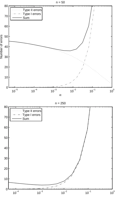
Although this bound was found too loose for practical use, we can model the Type I and Type II error rate as a function ofαfor artificial problems whose sparseness and regression weights are known. This is shown in Figure 3 for a specific instance of an Alarm data set (see Section 5 for details on this network) with two different sample sizes, n=50 (left) and n=250 (right). We did not use this information to tuneα in the experiments, as it cannot be obtained without prior knowledge, but the curves showed that anαinversely proportional to d(d−1)/2 has the same order of magnitude as the optimalαon the data sets we analyzed.

What we also see is that the Type I error curve rapidly goes up, whereas the Type II error curve is upper-bounded by the total number of links in the original graph. In terms of pure number of errors, setting a lowαwill thus be more beneficial than setting a higherαto get a lowβ. It is worth discussing, however, depending on the particular problem to solve, which is more desirable: missing causal links or getting extra causal links. In terms of Bayesian networks, getting too few links prevents the model from being able to reconstruct the full joint probability distribution, because we lose the I-map property; whereas getting too many links implies having to estimate more parameters from the same data and thus complexifies a subsequent parameter learning task.

4.3 The TCbwAlgorithm

Despite correctness of TC, with a low number of samples n it fails to have enough evidence for rejecting the null hypothesis of zero regression weight, and thus misses links (see detailed results in Section 5), even for a highα. We now try to address this particular issue by successively eliminating the most insignificant predictors and reevaluating the remaining ones. This is actually a backward stepwise-regression method. Pseudocode for this heuristics is listed in Algorithm 7.

Algorithm 7 The Total Conditioning Backward Feature-Selection Step 1: procedure TCBWFEATURESELECTION

2: P←V\X /* all predictors */

3: S← /0 /* significant predictors */ 4: while P6= /0and P6=S do

5: b←weights of P in the problem of regressing X on P

6: S←S∪ {predictors whose b weight is significant}

7: P←P\ {the p less significant predictors}

8: end while 9: return S 10: end procedure

(22)

10−5 10−4 10−3 10−2 10−1 100 0

10 20 30 40 50 60 70 80

α

Number of errors

n = 50 Type II errors

Type I errors Sum

10−4 10−3 10−2 10−1 100 0

10 20 30 40 50 60 70 80

n = 250 Type II errors

Type I errors Sum

Figure 3: Expected Type I and II errors as a function ofα

This stepwise regression raises some issues; notably, Tibshirani (1994) argues that the repeated tests on non-changing data are biased and that the remaining b coefficients are too large. We thus expect TCbwto be biased and to include more false positives than TC. Ideally, one would need a criterion to predict when the additional false positives would outweigh the benefits of reducing the false negatives. Whether such a criterion, which would allow us to know a priori whether TC or TCbwshould be used, can be found, is an open question.

Solving a standard multiple regression problem with d predictors traditionally has complexity

O

(nd3). Na¨ıvely solving d−1 regression problems d times in the case p=1 would have a com-plexity of

O

(nd5). But we can avoid reinverting matrices in the inner loop of the stepwise regression thanks to the following result.

LetΣ=XT_{X be n times the correlation matrix R, where X is the n}_×_{d matrix representing a}

(23)

the t-tests. Suppose we find that variable X1 is the weakest predictor, and want to reevaluate the weights of the other predictors at line 5 of TCbw. Let X\ibe the data set where variable Xihas been

removed. Then we need the matrixΩ−1to solve the new problem, whereΩ=XT_\₁X_\1. As a special case of Strassen’s blockwise matrix inversion formula, we have:

Σ=

σ

11 cT

c Ω

=⇒ Σ−1₌



 

1

σ11−cTΩ−1c

− cTΩ−1

σ11−cTΩ−1c

− Ω−1c

σ11−cTΩ−1c

Ω−1₊ Ω−1ccTΩ−1

σ11−cTΩ−1c



 .

Letσi j = (Σ−1)i j and b=Ω−1_{c. Then b are the weights of the regression of X1}_{on X2}_,_{· · ·}_,_X

dand

can be computed without knowingΩ−1(Raveh, 1985), see (9). We have:

σ11₌₁_/(σ

11−cTb)

and,(Σ−1)\1being the matrixΣ−1where the first row and column have been removed,

(Σ−1₎

\1=Ω−1+bbT/(σ11−cTb). We can thus computeΩ−1givenΣ−1with complexity

O

(d2)as follows:

Ω−1_{= (Σ}−1₎

\1−σ11bbT. (12)

This trick is also used in TC to find the inverse correlation matrix of the predictors from the inverse correlation matrix of the whole variable set.

Equation (12) is implemented in TCbw such that we never need to invert another matrix again once Σ−1 has been obtained, and leads to a complexity of

O

(d2) for stepwise elimination of a predictor. In the most computationally expensive case p=1, this elimination of row and column of the inverse matrix is repeated at most d−2 for each variable, yielding a complexity of

O(

nd4)for the whole feature-selection step for all variables. The overall complexity of TCbwis then

O

(nd4+

d22α). We are only adding one complexity degree in d with respect to TC with the additional stepwise regression.

5. Experimental Results

In this section, we report on experiments and results on two points separately. First, we test our procedure described in Algorithm 2 to recover the local structure with the collider set search given all Markov blankets, and compare it to the relevant steps of the GS algorithm, which are listed in Algorithm 1, with 5 different network topologies. For the sake of comparison, we also run the reference PC algorithm (Spirtes et al., 2001), initialized with the moral graph instead of the fully connected graph.

(24)

5.1 Experimental Setup

In order to test the accuracy of the various algorithms, we chose to sample data from the following known networks, from the Bayes net repository (Elidan, 2001):

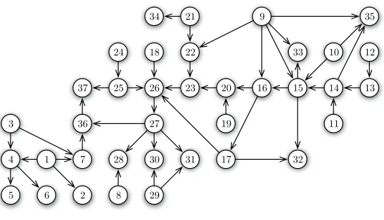
• Alarm network (Beinlich et al., 1989). This network has become a de facto standard bench-mark for structure-learning algorithms: it contains 37 nodes, 46 arcs, 4 undirected in the PDAG of the equivalence class. It was originally designed to help interpret monitoring data to alert anesthesiologists to various situations in the operating room. It is depicted in Figure 4.

• Insurance (Binder et al., 1997), 27 nodes, 52 arcs, 18 undirected in its PDAG. It was designed to evaluate car insurance risks. This network has fewer nodes than Alarm but is denser, see Figure 5.

• Hailfinder (Abramson et al., 1996), 56 nodes, 66 arcs, 17 undirected in its PDAG. It is a normative system that forecasts severe summer hail in northeastern Colorado. See Figure 6.

• Carpo,1061 nodes, 74 arcs, 24 undirected in its PDAG. It is meant to help diagnose the carpal tunnel syndrome. The version we used has three disconnected subgraphs, one of which is a single variable, and a relatively flat causal structure, as can be seen in Figure 7.

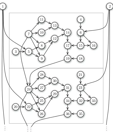
• A subset of Diabetes (Andreassen et al., 1991) with 104 nodes, 149 arcs, 8 undirected in its PDAG, which was designed as a preliminary model for insulin dose adjustment. This subset is made of 6 repeating patterns (there are 24 in the original network) of 17 nodes, plus 2 external nodes linked to every pattern. The first two of these patterns are shown in Figure 8.

We performed three series of experiments.

1. We compared our algorithm resolving the Markov blanket to the relevant steps of the Grow-Shrink algorithm, as described in Section 3.2, and to PC;

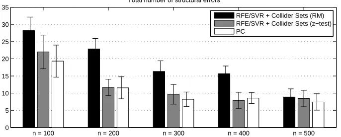
2. We tested the RFE-based approach and compared it to PC;

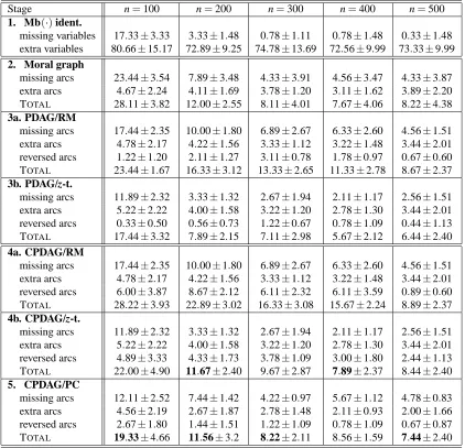
3. Finally, we compared TC and TCbwto three reference algorithms and examine their accuracy, run time, and number of tests while varying the network structure, the network size, and the sample size.

The chosen reference algorithms are:

1. The PC algorithm. PC is, like TC and TCbw, exponential in the worst case, when graphs are not sparse enough: we discuss which structural elements make PC or TC exhibit the exponential behavior;

2. The full Grow-Shrink algorithm, as described in Margaritis and Thrun (1999);

(25)

1 2 6 5 4 3 7 36 37 25 24 26 18 23 22 21 34 27 28 8 30 31 29 20 19 17 16 15 32 9 33 10 35 14 13 11 12

Figure 4: The Alarm network

1 2 4 3 5 7 6

8 9 11

10 14 13 12 15 16 17 18 22 20 19 23 21 24 25 26 27

Figure 5: The Insurance network

1 2 6 5 4 3 7 36 37 25 24 26 18 23 22 21 34 27 28 8 30 31 29 20 19 17 16 15 32 9 33 10 35 14 13 11 12 39 38 40 41 42 43 44 45 46 47 50 49

48 51 52

53

54