Learning Transformations for Clustering and Classification

(1)

Learning Transformations for Clustering and Classification

Qiang Qiu [email protected]

Department of Electrical and Computer Engineering Duke University

Durham, NC 27708, USA

Guillermo Sapiro [email protected]

Department of Electrical and Computer Engineering Department of Computer Science

Department of Biomedical Engineering Duke University

Durham, NC 27708, USA

Editor:Ben Recht

Abstract

A low-rank transformation learning framework for subspace clustering and classification is proposed here. Many high-dimensional data, such as face images and motion sequences, approximately lie in a union of low-dimensional subspaces. The corresponding subspace clustering problem has been extensively studied in the literature to partition such high-dimensional data into clusters corresponding to their underlying low-high-dimensional subspaces. Low-dimensional intrinsic structures are often violated for real-world observations, as they can be corrupted by errors or deviate from ideal models. We propose to address this by learning a linear transformation on subspaces using nuclear norm as the modeling and opti-mization criteria. The learned linear transformation restores a low-rank structure for data from the same subspace, and, at the same time, forces a maximally separated structure for data from different subspaces. In this way, we reduce variations within the subspaces, and increase separation between the subspaces for a more robust subspace clustering. This proposed learned robust subspace clustering framework significantly enhances the perfor-mance of existing subspace clustering methods. Basic theoretical results presented here help to further support the underlying framework. To exploit the low-rank structures of the transformed subspaces, we further introduce a fast subspace clustering technique, which efficiently combines robust PCA with sparse modeling. When class labels are present at the training stage, we show this low-rank transformation framework also significantly enhances classification performance. Extensive experiments using public data sets are presented, showing that the proposed approach significantly outperforms state-of-the-art methods for subspace clustering and classification. The learned low cost transform is also applicable to other classification frameworks.

Keywords: subspace clustering, classification, low-rank transformation, nuclear norm, feature learning

1. Introduction

(2)

handwritten images of a digit (Hastie and Simard, 1998), and trajectories of a moving object (Tomasi and Kanade, 1992) can all be well-approximated by a low-dimensional subspace of the high-dimensional ambient space. Thus, multiple class data often lie in a union of

low-dimensional subspaces. The ubiquitous subspace clustering problem is to partition

high-dimensional data into clusters corresponding to their underlying subspaces.

Standard clustering methods such as k-means in general are not applicable to subspace clustering. Various methods have been recently suggested for subspace clustering, such as Sparse Subspace Clustering (SSC) (Elhamifar and Vidal, 2013), and its extensions (Liu et al., 2010; Soltanolkotabi and Candes, 2012; Soltanolkotabi et al., 2013; Wang and Xu, 2013), Local Subspace Affinity (LSA) (Yan and Pollefeys, 2006), Local Best-fit Flats (LBF) (Zhang et al., 2012), Generalized Principal Component Analysis (Vidal et al., 2003), Ag-glomerative Lossy Compression (Ma et al., 2007), Locally Linear Manifold Clustering (Goh and Vidal, 2007), and Spectral Curvature Clustering (Chen and Lerman, 2009). A recent survey on subspace clustering can be found in Vidal (2011).

Low-dimensional intrinsic structures, which enable subspace clustering, are often vio-lated for real-world data. For example, under the assumption of Lambertian reflectance, Basri and Jacobs (2003) show that face images of a subject obtained under a wide variety of lighting conditions can be accurately approximated with a 9-dimensional linear subspace. However, real-world face images are often captured under pose variations; in addition, faces

are not perfectly Lambertian, and exhibit cast shadows and specularities (Cand`es et al.,

2011). Therefore, it is critical for subspace clustering to handle corrupted underlying struc-tures of realistic data, and as such, deviations from ideal subspaces.

When data from the same low-dimensional subspace are arranged as columns of a single matrix, the matrix should be approximately low-rank. Thus, a promising way to handle corrupted data for subspace clustering is to restore such low-rank structure. Recent efforts have been invested in seeking transformations such that the transformed data can be de-composed as the sum of a low-rank matrix component and a sparse error one (Peng et al., 2010; Shen and Wu, 2012; Zhang et al., 2011). Peng et al. (2010) and Zhang et al. (2011) are proposed for image alignment, Kuybeda et al. (2013) for the extension to multiple-classes with applications in cryo-tomograhy, and Shen and Wu (2012) is discussed in the context of salient object detection. All these methods build on recent theoretical and computational advances in rank minimization.

In this paper, we propose to improve subspace clustering and classification by learning a linear transformation on subspaces using matrix rank, via its nuclear norm convex surrogate, as the optimization criteria. The learned linear transformation recovers a low-rank structure for data from the same subspace, and, at the same time, forces a maximally separated structure for data from different subspaces (actually high nuclear norm, which as discussed later, improves the separation between the subspaces). In this way, we reduce variations within the subspaces, and increase separations between the subspaces for more accurate subspace clustering and classification.

(3)

are more visually similar in the new transformed space, enabling better face clustering and classification across pose.

This paper makes the following main contributions:

• Subspace low-rank transformation (LRT) is introduced and analyzed in the context

of subspace clustering and classification;

• A Learned Robust Subspace Clustering framework (LRSC) is proposed to enhance

existing subspace clustering methods;

• A discriminative low-rank (nuclear norm) transformation approach is proposed to

reduce the variation within the classes and increase separations between the classes for improved classification;

• We propose a specific fast subspace clustering technique, called Robust Sparse

Sub-space Clustering (R-SSC), by exploiting low-rank structures of the learned trans-formed subspaces;

• We discuss online learning of subspace low-rank transformation for big data;

• We demonstrate through extensive experiments that the proposed approach

signifi-cantly outperforms state-of-the-art methods for subspace clustering and classification.

The proposed approach can be considered as a way of learning data features, with such features learned in order to reduce within-class rank (nuclear norm), increase between class separation, and encourage robust subspace clustering. As such, the framework and criteria introduced here can be incorporated into other data classification and clustering problems.

In Section 2, we formulate and analyze the low-rank transformation learning problem. In Sections 3 and 4, we discuss the low-rank transformation for subspace clustering and classification respectively. Experimental evaluations are given in Section 5 on public data sets commonly used for subspace clustering evaluation. Finally, Section 6 concludes the paper.

2. Learning Low-rank Transformations (LRT)

Let {Sc}Cc=1 beC m-dimensional subspaces of Rd (not all subspaces are necessarily of the

same dimension, this is only assumed here to simplify notation). A data set is denoted as

Y = {y_i}N

i=1 ⊆ Rd, with each data point yi in one of the C subspaces and arranged as

a column of Y. Yc denotes the set of points in the c-th subspace Sc, points arranged as

columns of the matrix Yc.

As data points inYclie in a low-dimensional subspace, the matrixYcis expected to be

low-rank, and such low-rank structure is critical for accurate subspace clustering. However, as discussed above, this low-rank structure is often violated for real data.

(4)

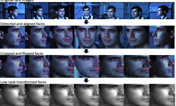
Original face images

Detected and aligned faces

Cropped and flipped faces

Low-rank transformed faces

Figure 1: Learned low-rank transformation on faces across pose. In the second row, the input faces are first detected and aligned, e.g., using the method in Zhu and Ramanan (2012). Pose models defined in Zhu and Ramanan (2012) enable an optional crop-and-flip step to retain the more informative side of a face in the third row. Our proposed approach learns linear transformations for face images to restore for the same subject a low-dimensional structure as shown in the last row. By comparing the last row to the first row, we can easily notice that faces from the same subject across different poses are more visually similar in the new transformed space, enabling better face clustering or recognition across pose (note that the goal is clustering/recognition and not reconstruction).

2.1 Preliminary Pedagogical Formulation using Rank

We first assume the data cluster labels are known beforehand, and this assumption is removed when discussing the full clustering approach in Section 3. We adopt matrix rank as the key learning criterion (presented here first for pedagogical reasons, to be later replaced by the nuclear norm), and compute one global linear transformation on all subspaces as

arg

T

min

C

X

c=1

rank(TYc)−rank(TY), s.t.||T||2 = 1, (1)

whereT∈Rd×d is one global linear transformation on all data points (we will later discuss

then T’s dimension is less than d), ||·||₂ denotes the matrix induced 2-norm, and γ is a

positive constant. Intuitively, minimizing the first representation term PC

c=1rank(TYc)

encourages a consistent representation for the transformed data from the same subspace;

and minimizing the second discrimination term −rank(TY) encourages a diverse

repre-sentation for transformed data from different subspaces (we will later formally discuss that the convex surrogate nuclear norm actually has this desired effect). The normalization

(5)

We now explain that the pedagogical formulation in (1) using rank is however not opti-mal to simultaneously reduce the variation within the same class subspaces and introduce separations between the different class subspaces, motivating the use of the nuclear norm

not only for optimization reasons but for modeling ones as well. Let A and B be

matri-ces of the same dimensions (standing for two classes Y1 and Y2 respectively), and [A,B]

(standing for Y) be the concatenation ofA and B, we have (Marsaglia and Styan, 1972)

rank([A,B])≤rank(A) +rank(B), (2)

with equality if and only ifAandBare disjoint, i.e., they intersect only at the origin (often

the analysis of subspace clustering algorithms considers disjoint spaces, e.g., Elhamifar and Vidal (2013)).

It is easy to show that (2) can be extended for the concatenation of multiple matrices,

rank([Y1,Y2,Y3,· · ·,YC])≤rank(Y1) +rank([Y2,Y3,· · · ,YC]) (3)

≤rank(Y1) +rank(Y2) +rank([Y3,· · ·,YC])

. . .

≤ C

X

c=1

rank(Yc),

with equality if matrices are independent. Thus, for (1), we have

C

X

c=1

rank(TYc)−rank(TY)≥0, (4)

and the objective function (1) reaches the minimum 0 if matrices are independent after

applying the learned transformation T. However, independence does not infer maximal

separation, an important goal for robust clustering and classification. For example, two lines intersecting only at the origin are independent regardless of the angle in between, and

they are maximally separated only when the angle becomes π₂. With this intuition in mind,

we now proceed to describe our proposed formulation based on the nuclear norm.

2.2 Problem Formulation using Nuclear Norm

Let ||A||∗ denote the nuclear norm of the matrixA, i.e., the sum of the singular values of

A. The nuclear norm ||A||∗ is the convex envelop ofrank(A) over the unit ball of matrices

Fazel (2002). As the nuclear norm can be optimized efficiently, it is often adopted as the best convex approximation of the rank function in the literature on rank optimization, e.g.,

Cand`es et al. (2011) and Recht et al. (2010).

One factor that fundamentally affects the performance of subspace clustering and clas-sification algorithms is the distance between subspaces. An important notion to quantify

the distance (separation) between two subspaces S_i and S_j is the smallest principal angle

θij (Miao and Ben-Israel, 1992; Elhamifar and Vidal, 2013), which is defined as

θij = min

u∈Si,v∈Sj

arccos u

0_v

(6)

0 0.1 0.2 0.3 0.4 0.5 0.6 0.7 0.8 0.9 1 0 0.1 0.2 0.3 0.4 0.5 0.6 0.7 0.8 0.9

1 Original subspaces

(a) θAB= π

2 = 1.57.

0 0.1 0.2 0.3 0.4 0.5 0.6 0.7 0.8 0.9 1 0 0.1 0.2 0.3 0.4 0.5 0.6 0.7 0.8 0.9

1 Transformed subspaces

(b) T=

1.00 0 0 1.00

;

θAB= 1.57.

0 0.1 0.2 0.3 0.4 0.5 0.6 0.7 0.8 0.9 1 0 0.1 0.2 0.3 0.4 0.5 0.6 0.7 0.8 0.9

(c)θAB=π

4 = 0.79,

|A|∗= 1,|B|∗= 1, |[A,B]|∗= 1.41

0 0.05 0.1 0.15 0.2 0.25 0.3 0.35 0.4 0.45 0.5 −0.2 −0.1 0 0.1 0.2 0.3 0.4

0.5 Transformed subspaces

(d)T=

0.50 −0.21 −0.21 0.91

;

θAB= 1.57, |A|∗= 1,|B|∗= 1, |[A,B]|∗= 1.95

0 0.2 0.4 0.6 0.8 1 0 0.2 0.4 0.6 0.8 1 −0.2 0 0.2 0.4 0.6 0.8 Original subspaces (e)

θAB= 0.79, θAC= 0.79, θBC= 1.05

A= 0.0141, B= 0.0131, C= 0.0148

,

|A|∗= 4.06, |B|∗= 4.08, |C|∗= 4.16.

−0.2 0 0.2 0.4 0.6 −0.2 0 0.2 0.4 0.6 −0.25 −0.2 −0.15 −0.1 −0.05 0 0.05 0.1 0.15 0.2 0.25 Transformed subspaces

(f)T=





0.39 −0.16 −0.16 −0.13 0.90 0.11 −0.23 0.11 0.57



;

θAB= 1.51, θAC = 1.49, θBC= 1.57

A= 0.0091, B= 0.0085, C= 0.0114

,

|A|∗= 1.93, |B|∗= 2.37, |C|∗= 1.20.

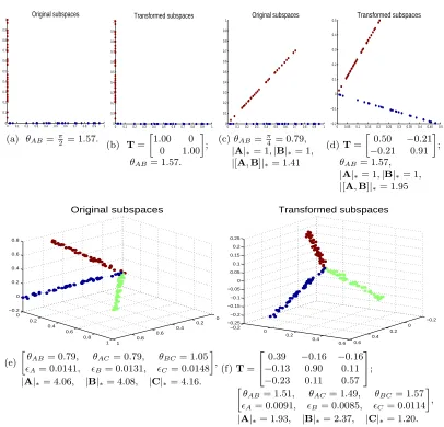
Figure 2: The learned transformationTusing (6) with the nuclear norm as the key criterion.

Three subspaces inR3 are denoted asA(red),B(blue),C(green). We denote the

angle between subspaces A and B as θAB (and analogous for the other pairs

of subspaces). Using (6), we transform A, B, C in (a),(c),(e) to (b),(d),(f)

respectively (in the first row the subspace C is empty, being this basically a

two dimensional example). Data points in (e) are associated with random noises

∼ N(0,0.01). We denote the root mean square deviation of points inAfrom the

true subspace asA(and analogous for the other subspaces). We observe that the

learned transformationTmaximizes the distance between every pair of subspaces

towards π₂, and reduces the deviation of points from the true subspace when

noise is present, note how the individual subspaces nuclear norm is significantly

reduced. Note that, in (c) and (d), we have the same rank values rank(A) =

(7)

Note thatθij ∈[0,π₂].We replace the rank function in (1) with the nuclear norm,

arg

T

min

C

X

c=1

||TYc||∗− ||TY||∗, s.t.||T||2 = 1. (6)

The normalization condition ||T||2 = 1 prevents the trivial solution T = 0. However,

understanding the effects of adopting a different normalization norm here is interesting and is the subject of future research.

It is important to note that (6) is not simply a relaxation of (1). Not only the replacement of the rank by the nuclear norm is critical for optimization considerations in reducing the variation within same class subspaces, but as we show next, the learned transformation

T using the objective function (6) also maximizes the separation between different class

subspaces (a missing property in (1)), leading to improved clustering and classification performance.

We start by presenting some basic norm relationships for matrices and their correspond-ing concatenations.

Theorem 1 Let A and B be matrices of the same row dimensions, and [A,B] be the concatenation of A and B, we have

||[A,B]||∗ ≤ ||A||∗+||B||∗.

Proof: See Appendix A.

Theorem 2 Let A and B be matrices of the same row dimensions, and [A,B] be the concatenation of A and B, we have

||[A,B]||∗ =||A||∗+||B||∗.

when the column spaces of A and B are orthogonal.

Proof: See Appendix B.

It is easy to see that theorems 1 and 2 can be extended for the concatenation of multiple matrices. Thus, for (6), we have,

C

X

c=1

||TY_c||∗− ||TY||∗ ≥0. (7)

Based on (7) and Theorem 2, the proposed objective function (6) reaches the minimum 0 if the column spaces of every pair of matrices are orthogonal after applying the learned

transformationT; or equivalently, (6) reaches the minimum 0 when the separation between

every pair of subspaces is maximized after transformation, i.e., the smallest principal angle

between subspaces equals π₂. Note that such improved separation is not obtained if the rank

(8)

We have then, both intuitively and theoretically, justified the selection of the criteria

(6) for learning the transform T. We now illustrate the properties of the learned

transfor-mation Tusing synthetic examples in Figure 2 (real examples are presented in Section 5).

Here we adopt a projected subgradient method described in Appendix C (though other modern nuclear norm optimization techniques could be considered, including recent real-time formulations Sprechmann et al. (2012)) to search for the transformation matrix T

that minimizes (6). As shown in Figure 2, the learned transformation Tvia (6) maximizes

the separation between every pair of subspaces towards π₂, and reduces the deviation of

the data points to the true subspace when noise is present. Note that, comparing Fig-ure 2c to FigFig-ure2d, the learned transformation using (6) maximizes the angle between

subspaces, and the nuclear norm changes from |[A,B]|∗ = 1.41 to|[A,B]|∗ = 1.95 to make

|A|∗ +|B|∗ − |[A,B]|∗ ≈ 0; However, in both cases, where subspaces are independent,

rank([A,B]) = 2, and rank(A) +rank(B)−rank([A,B]) = 0.

2.3 Comparisons with other Transformations

For independent subspaces, a transformation that renders them pairwise orthogonal can

be obtained in a closed-form as follows: we take a basis Uc for the column space of Yc

for each subspace, form a matrix U = [U1, ...,UC], and then obtain the orthogonalizing

transformation as T = (U0U)−1U0. To further elaborate the properties of our learned

transformation, using synthetic examples, we compare with the closed-form orthogonalizing transformation in Figure 3 and with linear discriminant analysis (LDA) in Figure 4.

Two intersecting planes are shown in Figure 3a. Though subspaces here are neither independent nor disjoint, the closed-form orthogonalizing transformation still significantly

increases the angle between the two planes towards π₂ in Figure 3b (note that the angle for

the common line here is always 0). Note also that the closed-form orthogonalizing

transfor-mation is of sizer×d, whereris the sum of the dimension of each subspace, and we plot just

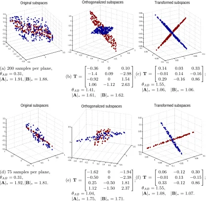
the first 3 dimensions for visualization. Comparing to the orthogonalizing transformation, our leaned transformation in Figure 3c introduces similar subspace separation, but enables significantly reduced within subspace variations, indicated by the decreased nuclear norm values (close to 1). The same set of experiments with different samples per subspace are shown in the second row of Figure 3. Our formulation in (6) not only maximizes the separa-tions between the different classes subspaces, but also simultaneously reduces the variasepara-tions within the same class subspaces.

Our learned transformation shares a similar methodology with LDA, i.e., minimizing

intra-class variation and maximizing inter-class separation. Two classes Y+ and Y− are

shown in Figure 4a, each class consisting of two lines. Our learned transformation in

Figure 4c shows smaller intra-class variation than LDA in Figure 4b by merging two lines

in each class, and simultaneously maximizes the angle between two classes towards π₂ (such

two-class clustering and classification is critical for example for trees-based techniques Qiu and Sapiro (2014)). Note that we usually use LDA to reduce the data dimension to the

number of classes minus 1; however, to better emphasize the distinction, we learn a (d−

1)×dsized transformation matrix using both methods. The closed-form orthogonalizing

transformation discussed above also gives higher intra-class variations as|Y+|∗ = 1.45 and

(9)

−0.5 0 0.5 −0.8 −0.6 −0.4 −0.2 0 0.2 0.4 0.6 −0.4 −0.3 −0.2 −0.1 0 0.1 0.2 0.3 Original subspaces

(a) 200 samples per plane,

θAB= 0.31,

|A|∗= 1.91,|B|∗= 1.88.

−1.5 −1 −0.5 0 0.5 1 1.5 −1 −0.5 0 0.5 1 −2 −1.5 −1 −0.5 0 0.5 1 1.5 Orthogonalized subspaces

(b) T=



  

−0.36 0 0.10 −1.4 0.09 −2.98 −0.92 0 1.54

1.06 −1.12 2.63



  

;

θAB= 1.41,

|A|∗= 1.61, |B|∗= 1.62.

−0.1 −0.05 0 0.05 0.1 −0.1 −0.05 0 0.05 0.1 −0.08 −0.06 −0.04 −0.02 0 0.02 0.04 0.06 0.08 Transformed subspaces

(c)T =





0.14 0.03 0.33 −0.01 0.14 −0.16

0.29 −0.16 0.86



;

θAB= 1.55,

|A|∗= 1.06, |B|∗= 1.06.

−1 −0.5 0 0.5 1 −0.5 0 0.5 1 −0.4 −0.3 −0.2 −0.1 0 0.1 0.2 0.3 Original subspaces

(d) 75 samples per plane,

θAB= 0.31,

|A|∗= 1.92,|B|∗= 1.81.

−0.8 _−0.6

−0.4 −0.2 0 0.2 0.4 _0.6

0.8 −0.5 0 0.5 −0.5 0 0.5 Orthogonalized subspaces

(e)T =



  

−1.62 0 −1.94 −0.50 0 −2.38 0.25 −0.50 1.81 1.12 −1.50 2.37



  

;

θAB= 1.04,

|A|∗= 1.75, |B|∗= 1.71.

−0.1 −0.05 0 0.05 0.1 −0.1 −0.05 0 0.05 0.1 −0.1 −0.05 0 0.05 0.1 0.15 Transformed subspaces

(f) T=





0.06 −0.12 0.30 −0.01 0.13 −0.15

0.33 −0.12 0.86



;

θAB= 1.55,

|A|∗= 1.08, |B|∗= 1.07.

Figure 3: Comparisons with the closed-form orthogonalizing transformation. Two inter-secting planes are shown in (a), and each plane contains 200 points. The closed-form orthogonalizing transclosed-formation significantly increase the angle between the

two planes towards π₂ in (b). Our leaned transformation in (c) introduces similar

(10)

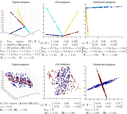
0 0.5 1 −0.5 0 0.5 1 0 0.1 0.2 0.3 0.4 0.5 0.6 0.7 0.8 0.9 Original subspaces

(a) Two classes {Y+,Y−},

Y+={A(blue),B(cyan)},

Y−={C(yellow),D(red)},

θAB= 1.1, θAC= 1.1, θAD= 1.1, θBC= 1.3, θBD= 1.4, θCD= 0.5

,

|Y+|∗= 1.58, |Y−|∗= 1.27.

−4 −3 −2 −1 0 1 2 3 4

−1 −0.5 0 0.5 1 1.5 2 2.5

3 LDA subspaces

(b)T=

−3.64 −1.95 5.98 0.19 3.87 3.35

;

θAB= 0.7, θAC= 0.78, θAD= 0.2, θBC= 1.5, θBD= 0.9, θCD= 0.57

,

|Y+|∗= 1.35, |Y−|∗= 1.27.

0 0.5 1 1.5

−1.4 −1.2 −1 −0.8 −0.6 −0.4 −0.2 0

(c)T=

1.47 0.26 −0.73 0.07 0.06 −1.62

;

θAB= 0.04, θAC= 1.54, θAD= 1.54, θBC= 1.55, θBD= 1.56, θCD = 0.01

,

|Y+|∗= 1.02, |Y−|∗= 1.00.

−0.5 0 0.5 −0.8 −0.6 −0.4 −0.2 0 0.2 0.4 0.6 −0.4 −0.3 −0.2 −0.1 0 0.1 0.2 0.3 Original subspaces

(d) Two classes{A(blue),B(red)},

θAB= 0.31,

|A|∗= 1.91,|B|∗= 1.88.

−3 −2 −1 0 1 2 3

−2.5 −2 −1.5 −1 −0.5 0 0.5 1 1.5

2 LDA subspaces

(e) T =

−0.54 2.60 −9.51 0.56 −3.21 −1.02

;

θAB= 0,

|A|∗= 1.52, |B|∗= 1.69.

−0.2 −0.15 −0.1 −0.05 0 0.05 0.1 0.15 0.2 0.25 −0.2 −0.15 −0.1 −0.05 0 0.05 0.1 0.15 0.2

(f) T =

0.49 −0.11 1.27 −0.09 0.29 −0.59

;

θAB= 1.57,

|A|∗= 1.08, |B|∗= 1.03.

Figure 4: Comparisons with the linear discriminant analysis (LDA). Two classes Y+ and

Y− are shown in (a), each class consisting of two lines. We notice that our

learned transformation (c) shows smaller intra-class variation than LDA in (b) by merging two lines in each class, and simultaneously maximizes the angle between

two classes towards π₂ (such two-class clustering and classification is critical for

(11)

intersecting planes, which cannot be improved by LDA, as shown in Figure 4e. However, our learned transformation in Figure 4f prepares the data to be separable using subspace clustering. As shown in Qiu and Sapiro (2014), the property demonstrated above makes our learned transformation a better learner than LDA in a binary classification tree.

Lastly, we generated an interesting disjoint case: we consider three lines A, B and C

on the same plane that intersect at the origin; the angles between them are θAB = 0.08,

θBC = 0.08, and θAC = 0.17. As the closed-form orthogonalizing approach is valid for

independent subspaces, it fails by producing θAB = 0.005, θBC = 0.005, θBC = 0.01. Our

framework is not limited to that, even if additional theoretical foundations are yet to come.

After our learned transformation, we have θAB = 1.20, θBC = 1.20, and θAC = 0.75. We

can make two immediate observations: First, all angles are significantly increased within the

valid range of [0,π₂]. Second,θAB+θBC+θAC =π(we made the same two observations while

repeating the experiments with different subspace angles). Though at this point we have no clean interpretation about how those angles are balanced when pair-wise orthogonality is not possible, we strongly believe that some theories are behind the above persistent observations and we are currently exploring this.

2.4 Discussions about Other Matrix Norms

We now discuss the advantages of replacing the rank function in (1) with the nuclear norm over other (popular) matrix norms, e.g., the induced 2-norm and the Frobenius norm.

Proposition 3 Let A and B be matrices of the same row dimensions, and [A,B] be the concatenation of A and B, we have

||[A,B]||₂ ≤ ||A||₂+||B||₂,

with equality if at least one of the two matrices is zero.

Proposition 4 Let A and B be matrices of the same row dimensions, and [A,B] be the concatenation of A and B, we have

||[A,B]||F ≤ ||A||F +||B||F, with equality if and only if at least one of the two matrices is zero.

We choose the nuclear norm in (6) for two major advantages that are not so favorable in other (popular) matrix norms:

• The nuclear norm is the best convex approximation of the rank function Fazel (2002),

which helps to reduce the variation within the subspaces (first term in (6));

• The objective function (6) is optimized when the distance between every pair of

sub-spaces is maximized after transformation, which helps to introduce separations be-tween the subspaces.

Note that (1), which is based on the rank, reaches the minimum when subspaces are independent but not necessarily maximally distant. Propositions 3 and 4 show that the property of the nuclear norm in Theorem 1 holds for the induced 2-norm and the Frobenius norm. However, if we replace the rank function in (1) with the induced 2-norm norm or the

Frobenius norm, the objective function is minimized at the trivial solutionT= 0, which is

(12)

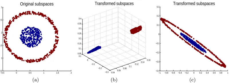
−0.5 0 0.5 1 1.5 2 0.5

1 1.5 2 2.5

(a)

0.04 0.06 0.08 0.1

0.12 0.14 0.16

−0.3 −0.2 −0.1 0 0.1 0.05 0.1 0.15 0.2 0.25 0.3 0.35 0.4

Transformed subspaces

(b)

−1 −0.8 −0.6 −0.4 −0.2 0 0.2 0.4 0.6 0.8 1 −0.4

−0.3 −0.2 −0.1 0 0.1 0.2 0.3

(c)

Figure 5: A synthetic example illustrating the kernelized transformation learning. (a) is transformed to (b) with an RBF kernel applied, and to (c) without kernel.

2.5 Online Learning Low-rank Transformations

When dataY is big, we use an online algorithm to learn the low-rank transformationT:

• We first randomly partition the data setY into B mini-batches;

• Using mini-batch subgradient descent, a variant of stochastic subgradient descent, the

subgradient in Appendix C is approximated by a sum of subgradients obtained from each mini-batch of samples,

T(t+1)=T(t)−ν

B

X

b=1

∆Tb, (8)

where ∆Tb is obtained using only data points in theb-th mini-batch;

• Starting with the first mini-batch, we learn the subspace transformationTb using data

only in theb-th mini-batch, with Tb−1 as warm restart.

2.6 Subspace Transformation with Compression

Given data Y ⊆ Rd, so far, we considered a square linear transformation T of size d×

d. If we devise a “fat” linear transformation T of size r×d, where (r < d), we enable

dimension reduction along with transformation. This connects the proposed framework with the literature on compressed sensing, though the goal here is to learn a “sensing”

matrix T for subspace classification and not for reconstruction Carson et al. (2012). The

nuclear-norm minimization provides a new metric for such compressed sensing design (or compressed feature learning) paradigm. Results with this reduced dimensionality will be presented in Section 5.

2.7 Kernelized Transformation

(13)

data points into an inner product space prior to learning the transformation. Given a data

point y, we create a nonlinear map K(y) = (κ(y,y1);...;κ(y,yn)) by computing the inner

product betweenyand a fixed set ofnpoints{y₁, ...,yn}randomly drawn from the training

set. The inner products are computed via the kernel function,κ(y,yi) =ϕ(y)0ϕ(yi), which

has to satisfy the Mercer conditions; note that no explicit representation for ϕis required.

Examples of kernel functions include polynomial kernelsκ(y,yi) = (y0yi+p)q (withp and

q being constants), and radial basis function (RBF) kernels κ(y,yi) = exp(−

||y−yi||22

2σ2 ) with

varianceσ2. Given a set of data pointsY, the set of mapped data is denoted asK(Y)⊆Rn.

We now learn ann×nkernelized transformation T minimizing

min

T

C

X

c=1

||TK(Yc)||∗− ||TK(Y)||∗, s.t.||T||2 = 1. (9)

Figure 5 shows a synthetic example illustrating the kernelized transformation learning, where a 256-dimensional RBF kernel is applied.

3. Subspace Clustering using Low-rank Transformations

We now move from classification, where we learned the transform from training labeled

data, to clustering, where no training data is available. In particular, we address the

sub-space clustering problem, meaning to partition the data setYintoCclusters corresponding to their underlying subspaces. We first present a general procedure to enhance the perfor-mance of existing subspace clustering methods in the literature. Then we further propose a specific fast subspace clustering technique to fully exploit the low-rank structure of (learned) transformed subspaces.

3.1 A Learned Robust Subspace Clustering (LRSC) Framework

In clustering tasks, the data labeling is of course not known beforehand in practice. The proposed algorithm, Algorithm 1, iterates between two stages: In the first assignment stage, we obtain clusters using any subspace clustering methods, e.g., SSC (Elhamifar and Vidal, 2013), LSA (Yan and Pollefeys, 2006), LBF (Zhang et al., 2012). In particular, in this paper we often use the new improved technique introduced in Section 3.2. In the second update stage, based on the current clustering result, we compute the optimal subspace transfor-mation that minimizes (6). The algorithm is repeated until the clustering assignments stop changing.

The LRSC algorithm is a general procedure to enhance the performance of any subspace clustering methods, and part of the beauty of the proposed model is that it can be applied to any such algorithm, and even beyond (Qiu and Sapiro, 2014). We don’t enforce an overall objective function at the present form for such versatility purpose.

To study convergence, one way is to adopt the subspace clustering method for the LRSC assignment step by optimizing the same LRSC update criterion (6): given the cluster

assignment and the transformationTat the current LRSC iteration, we take a pointyiout

of its current cluster (keep the rest assignments no change) and place it into a cluster Yc

that minimize PC

(14)

Tusing currentTas warm restart. In this way, we decrease (or keep) the overall objective function (6) after each LRSC iteration.

However, the above approach is computational expensive and only allow one specific subspace clustering method. Thus, in the present implementation, an overall objective function of the type that the LRSC algorithm optimizes can take a form such as

arg

T,{Sc}C_c₌₁ min

C

X

c=1

X

yi∈Sc

||Tyi−PTYcTyi||

2 2+λ[

C

X

c=1

||TYc||∗− ||TY||∗], s.t.||T||2= 1,

(10)

whereYcdenotes the set of pointsyi in the c-th subspaceSc, andPTYc denotes the

projec-tion ontoTYc. The LRSC iterative algorithm optimize (10) through alternative

minimiza-tion (with a similar form as the popular k-means, but with a different data model and with the learned transform). While formally studying its convergence is the subject of future re-search, the experimental validation presented already demonstrates excellent performance, with LRSC just one of the possible applications of the proposed learned transform.

In all our experiments, we observe significant clustering error reduction in the first few LRSC iterations, and the proposed LRSC iterations enable significantly cleaner subspaces for all subspace clustering benchmark data in the literature. The intuition behinds the observed empirical convergence is that the update step in each LRSC iteration decreases the second term in (10) to a small value close to 0 as discussed in Section 2; at the same time, the updated transformation tends to reduce the intra-subspace variation, which further reduces the first cluster deviation term in (10) even with assignments derived from various subspace clustering methods.

Input: A set of data pointsY={yi}Ni=1⊆Rdin a union ofCsubspaces.

Output: A partition ofYintoCdisjoint clusters{Yc}Cc=1based on underlying subspaces.

begin

1. Initial a transformation matrixTas the identity matrix ;

repeat

Assignment stage:

2. Assign points inTYto clusters with any subspace clustering methods, e.g., the proposed R-SSC;

Update stage:

3. Obtain transformationTby minimizing (6) based on the current clustering result ; untilassignment convergence;

4. Return the current clustering result{Yc}Cc=1;

end

Algorithm 1:Learning a robust subspace clustering (LRSC) framework.

3.2 Robust Sparse Subspace Clustering (R-SSC)

(15)

1. For the transformed subspaces, we first recover their low-rank representation L by

performing a low-rank decomposition (11), e.g., using RPCA (Cand`es et al., 2011),1

arg

L,S

min||L||∗+β||S||1 s.t.TY=L+S. (11)

2. Each transformed point Ty_i is then sparsely decomposed over L,

arg

xi

minkTy_i−Lxik2₂ s.t.kxik0 ≤K, (12)

whereK is a predefined sparsity value (K > d). As explained in Elhamifar and Vidal

(2013), a data point in a linear or affine subspace of dimension d can be written as

a linear or affine combination of dord+ 1 points in the same subspace. Thus, if we

represent a point as a linear or affine combination of all other points, a sparse linear

or affine combination can be obtained by choosingdor d+ 1 nonzero coefficients.

3. As the optimization process for (12) is computationally demanding, we further simplify (12) using Local Linear Embedding (Roweis and Saul, 2000; Wang et al., 2010). Each

transformed pointTy_i is represented using itsK Nearest Neighbors (NN) inL, which

are denoted asLi,

arg

xi

minkTy_i−Lixik2₂ s.t.10xi= 1. (13)

Let Li¯ = Li −1TyT_i . xi can then be efficiently obtained in closed form (Saul and

Roweis, 2000),

xi =Li¯ L¯T_i \1,

wherex=A\B solves the system of linear equationsAx=B, and then we rescale

xiso that10xi= 1 . As suggested in Roweis and Saul (2000), if the correlation matrix

¯

LiL¯T_i is nearly singular, it can be conditioned by adding a small multiple of the identity

matrix. From experiments, we observe this simplification step dramatically reduces the running time, without sacrificing the accuracy.

4. Given the sparse representationxiof each transformed data pointTy_i, we denote the

sparse representation matrix as X= [x1. . .xN]. It is noted that xi is written as an

N-sized vector with no more thanK << Nnon-zero values (N being the total number

of data points). The pairwise affinity matrix is now defined asW=|X|+|XT_|_,_and

the subspace clustering is obtained using spectral clustering (Luxburg, 2007).

Based on experimental results presented in Section 5, the proposed R-SSC outperforms state-of-the-art subspace clustering techniques, in both accuracy and running time, e.g., about 500 times faster than the original SSC using the implementation provided in Elhamifar and Vidal (2013). Performance is further enhanced when R-SCC is used as an internal step of LRSC in Algorithm 1.

(16)

4. Classification using Single or Multiple Low-rank Transformations

In Section 2, learning one global transformation over all classes has been discussed, and then incorporated into a clustering framework in Section 3. The availability of data labels for training enables us to consider instead learning individual class-based linear transformation. The problem of class-based linear transformation learning can be formulated as

arg {Tc}Cc=1

min

C

X

c=1

[||T_cYc||∗−λ||TcY¬c||∗], (14)

where Tc∈ Rd×d denotes the transformation for the c-th class, Y¬c =Y\Yc denotes all

data except the c-th class, andλis a positive balance parameter.

When a global transformation matrix Tis learned, we can perform classification in the

transformed space by simply considering the transformed dataTY as the new features. For

example, when a Nearest Neighbor (NN) classifier is used, a testing sample y uses Ty as

the feature and searches for nearest neighbors among TY.

To fully exploit the low-rank structure of the transformed data, we propose to perform classification through the following procedure:

• For the c-th class, we first recover its low-rank representationLc by performing

low-rank decomposition (15), e.g., using RPCA (Cand`es et al., 2011):2

arg

Lc,Sc

min||L_c||∗+β||Sc||1 s.t.TYc=Lc+Sc. (15)

• Each testing imageywill then be assigned to the low-rank subspaceLcthat gives the

minimal reconstruction error through sparse decomposition, e.g., using OMP (Pati et al., Nov. 1993):

arg

x

minkTy−Lixk22 s.t.kxk0≤T, (16)

whereT is a predefined sparsity value.

When class-based transformations{Tc}C

c=1 are learned, we perform recognition in a similar

way. However, now we apply all the learned transforms Tc to each testing data point and

then pick the best one using the same criterion of minimal reconstruction error through sparse decomposition (16).

5. Experimental Evaluation

This section first presents experimental evaluations on subspace clustering using three public data sets (standard benchmarks): the MNIST handwritten digit data set, the Extended YaleB face data set (Georghiades et al., 2001) and the Hopkins 155 database of motion segmentation. The MNIST data set consists of 8-bit gray scale handwritten digit images of “0” through “9” and 7000 examples for each class. The Extended YaleB face data set

(17)

contains 38 subjects with near frontal pose under 64 lighting conditions. All the images are

resized to 16×16. The classical Hopkins 155 database of motion segmentation, which is

available athttp://www.vision.jhu.edu/data/hopkins155, contains 155 video sequences

along with extracted feature trajectories, where 120 of the videos have two motions and 35 of the videos have three motions.

Subspace clustering methods compared are SSC (Elhamifar and Vidal, 2013), LSA (Yan and Pollefeys, 2006), and LBF (Zhang et al., 2012). Based on the studies in Elhamifar and Vidal (2013), Vidal (2011) and Zhang et al. (2012), these three methods exhibit state-of-the-art subspace clustering performance. We adopt the LSA and SSC implementations provided

in Elhamifar and Vidal (2013) fromhttp://www.vision.jhu.edu/code/, and the LBF

im-plementation provided in Zhang et al. (2012) from _{http://www.ima.umn.edu/~zhang620/}

lbf/. We adopt similar setups as described in Zhang et al. (2012) for experiments on

subspace clustering.

This section then presents experimental evaluations on classification using two public face data sets: the CMU PIE data set (Sim et al., 2003) and the Extended YaleB data set. The PIE data set consists of 68 subjects imaged simultaneously under 13 different poses

and 21 lighting conditions. All the face images are resized to 20×20. We adopt a NN

classifier unless otherwise specified.

5.1 Subspace Clustering with Illustrative Examples

For illustration purposes, we conduct the first set of experiments on a subset of the MNIST data set. We adopt a similar setup as described in Zhang et al. (2012), using the same sets of 2 or 3 digits, and randomly choose 200 images for each digit. We set the sparsity value

K = 6 for R-SSC, and perform 100 iterations for the subgradient updates while learning the

transformation on subspaces. The subgradient update step wasν = 0.02 (see Appendix C

for details on the projected subgradient optimization algorithm).

Unless otherwise stated, we do not perform dimension reduction, such as PCA or ran-dom projections, to preprocess the data, thereby further saving computations (please note that the learned transform can itself reduce dimensions if so desired, see Section 5.8). In the literature, e.g., Elhamifar and Vidal (2013), Vidal (2011) and Zhang et al. (2012), pro-jection to a very low dimension is usually performed to enhance the clustering performance. However, it is often not obvious how to determine the correct projection dimension for real data, and many subspace clustering methods show sensitive to the choice of the projection dimension. This dimension reduction step is not needed in the framework proposed here.

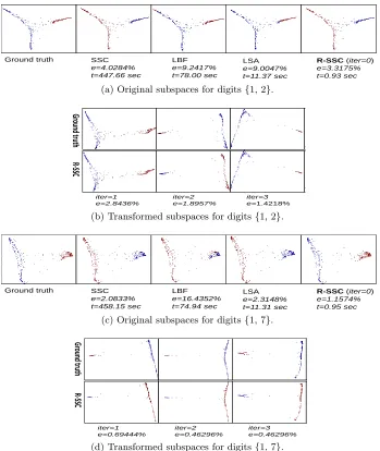
Figure 6 shows the misclassification rate (e) and running time (t) on clustering

(18)

LBF

e=9.2417% t=78.00 sec

Ground truth LSA

e=9.0047% t=11.37 sec

SSC

e=4.0284% t=447.66 sec

R-SSC (iter=0)

e=3.3175% t=0.93 sec

Unsupervised clustering digits [1 2] in MNIST (e: misclassification rate t: running time) R-SSC: Robust Sparse Subspace clustering (our approach)

(a) Original subspaces for digits{1, 2}.

Clustering digits [1 2] using low-rank subspace transformation (iter: EM iterations)

iter=1 e=2.8436%

iter=2 e=1.8957%

Grou

nd

truth

R-SSC

iter=3 e=1.4218%

iter=4 e=1.8957%

iter=5 e=1.8957%

(b) Transformed subspaces for digits{1, 2}.

LBF

e=16.4352% t=74.94 sec

Ground truth LSA

e=2.3148% t=11.31 sec

SSC

e=2.0833% t=458.15 sec

R-SSC (iter=0)

e=1.1574% t=0.95 sec

Unsupervised clustering digits [1 7] in MNIST (e: misclassification rate t: running time) R-SSC: Robust Sparse Subspace clustering (our approach)

(c) Original subspaces for digits{1, 7}.

Clustering digits [1 7] using low-rank subspace transformation (iter: EM iterations)

iter=1 e=0.69444%

iter=2 e=0.46296%

Grou

nd

truth

R-SSC

iter=3 e=0.46296%

iter=4 e=0.46296%

iter=5 e=0.46296%

(d) Transformed subspaces for digits{1, 7}.

Figure 6: Misclassification rate (e) and running time (t) on clustering 2 digits. Methods

compared are SSC Elhamifar and Vidal (2013), LSA Yan and Pollefeys (2006), and LBF Zhang et al. (2012). For visualization, the data are plotted with the dimension reduced to 2 using Laplacian Eigenmaps Belkin and Niyogi (2003).

Different clusters are represented by different colors and theground truthis

plot-ted with the true cluster labels. iterindicates the number of LRSC iterations in

(19)

LBF

e=30.9904%

Ground truth _LSA

e=30.1917%

Unsupervised clustering digits [1 2 3] in MNIST (e: misclassification rate)

R-LBF

e=9.5847%

Ground truth

R-LBF: adopt LBF as the subspace clustering method for transformed subspaces

Transformed subspaces Original subspaces

(a) Digits{1, 2, 3}.

LBF

e=35.0937%

Ground truth LSA

e=21.2947%

Unsupervised clustering digits [2 4 8] in MNIST (e: misclassification rate)

R-LBF

e=6.9847%

Ground truth

R-LBF: adopt LBF as the subspace clustering method for transformed subspaces

Transformed subspaces Original subspaces

(b) Digits{2, 4, 8}.

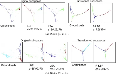
Figure 7: Misclassification rate (e) on clustering 3 digits. Methods compared are LSA

(20)

Subsets [0:1] [0:2] [0:3] [0:4] [0:5] [0:6] [0:7] [0:8]

C 2 3 4 5 6 7 8 9

LSA 0.47 47.57 36.73 30.90 40.46 48.13 39.87 44.03

LBF 0.47 23.62 29.19 51.37 48.99 53.01 39.87 38.79

LRSC 0 3.88 3.89 5.31 14.04 13.79 14.50 16.05

Table 1: Misclassification rate (e%) on clustering different numbers of digits in the MNIST

data set, [0 :c] denotes the subset ofc+ 1 digits from digit 0 toc. We randomly

pick 100 samples per digit. For all cases, the proposed LRSC method significantly outperforms state-of-the-art methods.

structure for data from the same subspace, but also increases the separations between the subspaces for more accurate clustering.

Figure 7 shows misclassification rate (e) on clustering subspaces of three digits. Here we

adopt LBF in our LRSC framework, denoted as Robust LBF (R-LBF), to illustrate that the performance of existing subspace clustering methods can be enhanced using the proposed LRSC algorithm. After convergence, R-LBF, which uses the proposed learned subspace transformation, significantly outperforms state-of-the-art methods.

Table 1 shows the misclassification rate on clustering different number of digits, [0 :c]

denotes the subset ofc+ 1 digits from digit 0 toc. We randomly pick 100 samples per digit

to compare the performance when a fewer number of data points per class are present. For all cases, the proposed LRSC method significantly outperforms state-of-the-art methods.

5.1.1 Online vs. Batch Learning

In this set of experiments, we use digits {1, 2} from the MNIST data set. We select

1000 images for each digit, and randomly partition them into 5 mini-batches. We first perform one iteration of LRSC in Algorithm 1 over all selected data with and without the norm constraint. As shown in Figure 8a, we both observe empirical convergence for subspace transformation learning via (6) using the projected subgradient method presented in Appendix C.

Starting with the first batch, we then perform one iteration of LRSC over one mini-batch a time, with the subspace transformation learned from the previous mini-mini-batch as warm restart. We adopt here 100 iterations for the subgradient descent updates. As shown in Figure 8b, we observe similar empirical convergence for online transformation learning.

To converge to the same objective function value, it takes 131.76 sec. for online learning

and 700.27 sec. for batch learning.

5.2 Application to Face Clustering

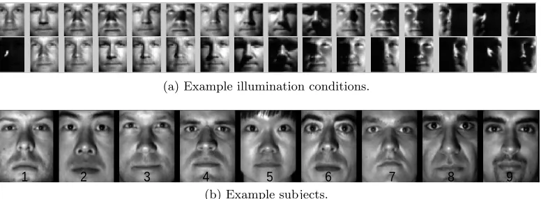
In the Extended YaleB data set, each of the 38 subjects is imaged under 64 lighting

condi-tions, shown in Figure 9a. Under the assumption of Lambertian reflectance, face images

of each subject under different lighting conditions can be accurately approximated with a

9-dimensional linear subspace (Basri and Jacobs, 2003). We conduct the face clustering

(21)

0 100 200 300 400 500 0

5 10 15 20 25

Number of Iterations

Objective Function

Norm free

||T||2= 1

(a) Batch learning.

0 100 200 300 400 500

0 5 10 15 20 25

Number of Iterations

O

bj

ec

tiv

e

Fu

nc

tio

n

Batch Online

(b) Online vs. batch learning (γ= 1).

Figure 8: Convergence of the objective function (6) using online and batch learning for sub-space transformation. We always observe empirical convergence for both online and batch learning. In (a), we learn with and without the norm constraint re-spectively. More discussions on convergence can be found in Appendix C. In (b),

to converge to the same objective function value, it takes 131.76 sec. for online

learning and 700.27 sec. for batch learning.

(a) Example illumination conditions.

1 2 3 4 5 6 7 8 9 (b) Example subjects.

(22)

−0.02 −0.015 −0.01 −0.005 0 0.005 0.01 0.015 0.02 0.025 0.03 −0.03

−0.02 −0.01 0 0.01 0.02 0.03

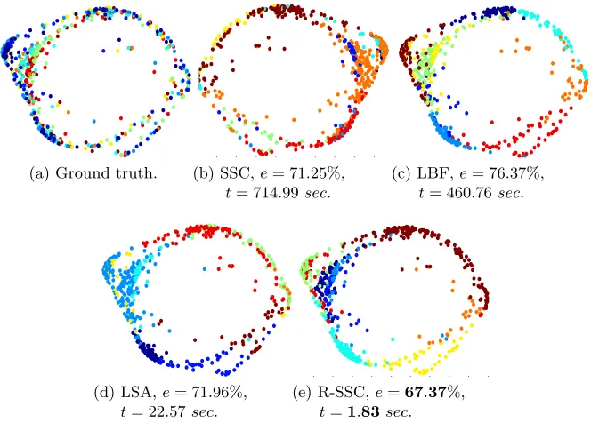
(a) Ground truth. −0.03 −0.025 −0.02 −0.015 −0.01 −0.005 0 0.005 0.01 0.015 0.02

−0.03 −0.02 −0.01 0 0.01 0.02 0.03

(b) SSC,e= 71.25%,

t= 714.99sec.

−0.02 −0.015 −0.01 −0.005 0 0.0050.01 0.015 0.02 0.025 0.03 −0.03

−0.02 −0.01 0 0.01 0.02 0.03

(c) LBF,e= 76.37%,

t= 460.76sec.

−0.02 −0.015 −0.01 −0.005 0 0.0050.01 0.015 0.02 0.0250.03 −0.03

−0.02 −0.01 0 0.01 0.02 0.03

(d) LSA,e= 71.96%,

t= 22.57sec.

−0.02 −0.015 −0.01 −0.005 0 0.0050.01 0.015 0.02 0.025 0.03 −0.03

−0.02 −0.01 0 0.01 0.02 0.03

(e) R-SSC,e=67.37%,

t=1.83sec.

Figure 10: Misclassification rate (e) and running time (t) on clustering 9 subjects using

(23)

−0.05 −0.04 −0.03 −0.02 −0.01 0 0.01 0.02 −0.05 −0.04 −0.03 −0.02 −0.01 0 0.01 0.02 0.03

(a) Ground truth (iter=1).−0.05−0.05 −0.04 −0.03 −0.02 −0.01 0 0.01 0.02 −0.04 −0.03 −0.02 −0.01 0 0.01 0.02 0.03

(b)e= 40.39% (iter=1).−0.04−0.04 −0.03 −0.02 −0.01 0 0.01 0.02 0.03 0.04 −0.03 −0.02 −0.01 0 0.01 0.02 0.03

(c) Ground truth (iter=2).−0.04−0.04 −0.03 −0.02 −0.01 0 0.01 0.02 0.03 0.04 −0.03 −0.02 −0.01 0 0.01 0.02 0.03

(d)e= 33.51% (iter=2).

−0.05 −0.04 −0.03 −0.02 −0.01 0 0.01 0.02 0.03 −0.03 −0.02 −0.01 0 0.01 0.02 0.03 0.04

(e) Ground truth (iter=3).−0.03−0.05 −0.04 −0.03 −0.02 −0.01 0 0.01 0.02 0.03 −0.02 −0.01 0 0.01 0.02 0.03 0.04

(f)e= 29.98% (iter=3).−0.04−0.03 −0.02 −0.01 0 0.01 0.02 0.03 0.04 0.05 −0.03 −0.02 −0.01 0 0.01 0.02 0.03

(g) Ground truth (iter=6).−0.04−0.03 −0.02 −0.01 0 0.01 0.02 0.03 0.04 0.05 −0.03 −0.02 −0.01 0 0.01 0.02 0.03

(h)e= 13.40% (iter=6).

−0.02 −0.01 0 0.01 0.02 0.03 0.04 0.05 −0.02 −0.01 0 0.01 0.02 0.03 0.04

(i) Ground truth (iter=8).−0.02 −0.01 0 0.01 0.02 0.03 0.04 0.05

−0.02 −0.01 0 0.01 0.02 0.03 0.04

(j)e= 6.17% (iter=8).−0.01 0 0.01 0.02 0.03 0.04 0.05

−0.04 −0.03 −0.02 −0.01 0 0.01 0.02

(k) Ground truth (iter=12).

−0.01 0 0.01 0.02 0.03 0.04 0.05 −0.04 −0.03 −0.02 −0.01 0 0.01 0.02

(l)e=4.94% (iter=12).

0 2 4 6 8 10 12

0 10 20 30 40 50 60 70

Number of LRSC Iterations

Misclassification Rate

(m) Misclassification rate.

0 20 40 60 80 100

−0.5 0 0.5 1 1.5 2 2.5 3 3.5 4

Number of Iterations

Objective Function iter=1 iter=2 iter=3 iter=4 iter=5 iter=6

(n) Convergence ofTupdating

Figure 11: Misclassification rate (e) on clustering 9 subjects using the proposed LRSC

framework. We adopt the proposed R-SSC technique for the clustering step. With the proposed LRSC framework, the clustering error of R-SSC is further

reduced significantly, e.g., from 67.37% to 4.94% for the 9-subject case. Note

(24)

.00 .10 .05 .07 .11 .07 .07 .10 .09

.10 .00 .08 .10 .11 .07 .09 .09 .11

.05 .08 .00 .07 .13 .09 .08 .09 .09

.07 .10 .07 .00 .13 .09 .04 .10 .09

.11 .11 .13 .13 .00 .11 .11 .13 .13

.07 .07 .09 .09 .11 .00 .08 .08 .08

.07 .09 .08 .04 .11 .08 .00 .09 .10

.10 .09 .09 .10 .13 .08 .09 .00 .07

.09 .11 .09 .09 .13 .08 .10 .07 .00 s1 s2 s3 s4 s5 s6 s7 s8 s9

s1 s2 s3 s4 s5 s6 s7 s8 s9

(a) Original smallest angles.

.00 .26 .20 .20 .29 .20 .24 .22 .21

.26 .00 .26 .26 .34 .26 .30 .27 .24

.20 .26 .00 .24 .34 .22 .25 .19 .24

.20 .26 .24 .00 .35 .18 .23 .25 .25

.29 .34 .34 .35 .00 .33 .32 .29 .31

.20 .26 .22 .18 .33 .00 .21 .21 .23

.24 .30 .25 .23 .32 .21 .00 .26 .23

.22 .27 .19 .25 .29 .21 .26 .00 .24

.21 .24 .24 .25 .31 .23 .23 .24 .00 s1 s2 s3 s4 s5 s6 s7 s8 s9

s1 s2 s3 s4 s5 s6 s7 s8 s9

(b) Transformed smallest angles.

1.0 .64 .64 .69 .67 .63 .58 .72 .67

.64 1.0 .63 .62 .64 .65 .61 .62 .63

.64 .63 1.0 .66 .65 .64 .61 .67 .65

.69 .62 .66 1.0 .64 .64 .61 .68 .67

.67 .64 .65 .64 1.0 .64 .57 .70 .67

.63 .65 .64 .64 .64 1.0 .59 .67 .70

.58 .61 .61 .61 .57 .59 1.0 .61 .61

.72 .62 .67 .68 .70 .67 .61 1.0 .66

.67 .63 .65 .67 .67 .70 .61 .66 1.0

s1 s2 s3 s4 s5 s6 s7 s8 s9

(c) Original mean cosine angles.

1.0 .47 .47 .52 .49 .44 .42 .51 .47

.47 1.0 .46 .45 .47 .48 .45 .44 .44

.47 .46 1.0 .48 .47 .45 .43 .47 .45

.52 .45 .48 1.0 .48 .47 .46 .49 .47

.49 .47 .47 .48 1.0 .47 .42 .49 .46

.44 .48 .45 .47 .47 1.0 .42 .47 .50

.42 .45 .43 .46 .42 .42 1.0 .45 .43

.51 .44 .47 .49 .49 .47 .45 1.0 .46

.47 .44 .45 .47 .46 .50 .43 .46 1.0

s1 s2 s3 s4 s5 s6 s7 s8 s9

(d) Transformed mean cosine angles.

1 2 3 4 5 6 7 8 9 10 15 20 Subjects Nuclear Norm Original Transformed

(e) Subspace nuclear norm.

(25)

Subsets [1:10] [1:15] [1:20] [1:25] [1:30] [1:38]

C 10 15 20 25 30 38

LSA 78.25 82.11 84.92 82.98 82.32 84.79

LBF 78.88 74.92 77.14 78.09 78.73 79.53

LRSC 5.39 4.76 9.36 8.44 8.14 11.02

Table 2: Misclassification rate (e%) on clustering different number of subjects in the

Ex-tended YaleB face data set, [1 :c] denotes the first c subjects in the data set. For

all cases, the proposed LRSC method significantly outperforms state-of-the-art methods.

Methods Misclassification (%)

orthogonalizing 61.36

LDA 9.77

Proposed 5.47

Table 3: Misclassification rate (e%) on clustering 38 subjects in the Extended YaleB data set

using supervised transformation learning. The proposed transformation learning outperforms both the closed-form orthogonalizing transformation and LDA on clustering the transformed data.

for R-SSC, and perform 100 iterations for the subgradient descent updates while learning the transformation.

Figure 10 shows error rate (e) and running time (t) on clustering subspaces of 9 subjects

using different subspace clustering methods. The proposed R-SSC techniques outperforms state-of-the-art methods both in accuracy and running time. As shown in Figure 11, using the proposed LRSC algorithm (that is, learning the transform), the misclassification errors

of R-SSC are further reduced significantly, for example, from 67.37% to 4.94% for the 9

subjects. Figure 11n shows the convergence of the Tupdating step in the first few LRSC

iterations. The dramatic performance improvement can be explained in Figure 12. We observe, as expected from the theory presented before, that the learned subspace transfor-mation increases the distance (the smallest principal angle) between subspaces and, at the same time, reduces the nuclear norms of subspaces. More results on clustering subspaces of 2 and 3 subjects are shown in Figure 13.

Table 2 shows misclassification rate (e) on clustering subspaces of different number of

subjects, [1 :c] denotes the first c subjects in the extended YaleB data set. For all cases,

(26)

LBF e=49.2063% t= 76.19 sec

Ground truth LSA

e=50% t=1.22 sec SSC

e=47.619% t= 101.44 sec

R-SSC (iter=0) e=42.0635% t= 0.32 sec

[1 2] in YaleB

Original subspaces

(a) Subjects{1, 2}.

[1 2] in YaleB

R-SSC

e=0%

Ground truth

(b) Subjects{1, 2}.

LBF e=49.2063% t=70.79 sec

Ground truth LSA

e=46.8254% t=1.24 sec SSC

e=45.2381% t= 113.75 sec

R-SSC (iter=0) e=38.8889% t= 0.21 sec

[2 3] in YaleB

Original subspaces

(c) Subjects{2, 3}.

[2 3] in YaleB

R-SSC

e=2.381%

Ground truth

(d) Subjects{2, 3}.

LBF e= 64.0212% t=121.63 sec

Ground truth LSA

e=47.619% t=2.84 sec SSC

e=53.9683% t=180.88 sec

R-SSC (iter=0) e=41.2698% t= 0.29 sec

[4 5 6] in YaleB

Original subspaces

(e) Subjects{4, 5, 6}.

[4 5 6] in YaleB

R-SSC

e=4.2328%

Ground truth

(f) Subjects{4, 5, 6}.

LBF e=64.0212% t=119.28 sec

Ground truth LSA

e=65.0794% t=2.74 sec SSC

e=65.0794% t=186.36 sec

R-SSC (iter=0) e= 65.6085% t= 0.25 sec

[7 8 9] in YaleB

Original subspaces

(g) Subjects{7, 8, 9}.

[7 8 9] in YaleB

R-SSC

e= 1.5873%

Ground truth

(h) Subjects{7, 8, 9}.

Figure 13: Misclassification rate (e) and running time (t) on clustering 2 and 3 subjects.

(27)

Check Traffic Articulated All

Mean Median Mean Median Mean Median Mean Median

2-motion

LSA 2.57 0.27 5.43 1.48 4.10 1.22 3.45 0.59

LBF 1.59 0 0.20 0 0.80 0 1.16 0

SSC 1.12 0 0.02 0 0.62 0 0.82 0

LRSC 1.19 0 0.23 0 0.88 0 0.92 0

3-motion

LSA 5.80 1.77 25.07 23.79 7.25 7.25 9.73 2.33

LBF 4.57 0.94 0.38 0 2.66 2.66 3.63 0.64

SSC 2.97 0.27 0.58 0 1.42 0 2.45 0.2

LRSC 1.59 0 0.32 0 1.60 1.60 1.34 0

Table 4: Misclassification rate (e%) on two motions and three motions segmentation in the

Hopkins 155 data set. As shown in Vidal (2011); Zhang et al. (2012), the SSC method significantly outperforms all previous state-of-the-art methods on this data set. The proposed LRSC shows comparable results to SSC for two motions and outperforms SSC for three motions. Note that our method is orders of magnitude faster than SSC.

In Figure 3 and Figure 4, using synthetic examples, we previously compared our learned transformation with the closed-form orthogonalizing transformation and LDA. In Table 3, we further compare three transformations using real data. We perform supervised trans-formation learning on all 38 subjects in the Extended YaleB data set using three different transformation learning algorithms, and then perform subspace clustering on the trans-formed data. The proposed transformation learning significantly outperforms the other two methods.

5.3 Application to Motion Segmentation

(28)

Method Accuracy (%)

D-KSVD Zhang and Li (2010) 94.10

LC-KSVD Jiang et al. (2011) 96.70

SRC Wright et al. (2009) 97.20

Original+NN 91.77

Class LRT+NN 97.86

Class LRT+OMP 92.43

Global LRT+NN 99.10

Global LRT+OMP 99.51

Table 5: Recognition accuracies (%) under illumination variations for the Extended YaleB

data set. The recognition accuracy is increased from 91.77% to 99.10% by simply

applying the learned low-rank transformation (LRT) matrix to the original face images.

5.4 Application to Face Recognition across Illumination

For the Extended YaleB data set, we adopt a similar setup as described in Jiang et al. (2011); Zhang and Li (2010). We split the data set into two halves by randomly selecting 32 lighting conditions for training, and the other half for testing. We learn a global low-rank transformation matrix from the training data.

We report recognition accuracies in Table 5. We make the following observations. First,

the recognition accuracy is increased from 91.77% to 99.10% by simply applying the learned

transformation matrix to the original face images. Second, the best accuracy is obtained by first recovering the low-rank subspace for each subject, e.g., the third row in Figure 14a. Then, each transformed testing face, e.g., the second row in Figure 14b, is sparsely decom-posed over the low-rank subspace of each subject through OMP, and classified to the subject with the minimal reconstruction error. A sparsity value 10 is used here for OMP. As shown in Figure 14c, the low-rank representation for each subject shows reduced variations caused by illumination. Third, the global transformation performs better here than class-based transformations, which can be due to the fact that illumination in this data set varies in a globally coordinated way across subjects. Last but not least, our method outperforms state-of-the-art sparse representation based face recognition methods.

5.5 Application to Face Recognition across Pose

We adopt the similar setup as described in Castillo and Jacobs (2009) to enable the com-parison. In this experiment, we classify 68 subjects in three poses, frontal (c27), side (c05), and profile (c22), under lighting condition 12. We use the remaining poses as the training data.

(29)

Shared T YaleB train

Original face images

Low-rank components

Sparse errors

(a) Low-rank decomposition of globally transformed training samples

Shared T YaleB Test

Low-rank transformation

(b) Globally transformed testing samples

Shared T YaleB Test

(c) Mean low-rank components for subjects in the training data

Figure 14: Face recognition across illumination using global low-rank transformation.

Method Frontal Side Profile

(c27) (c05) (c22)

SMD Castillo and Jacobs (2009) 83 82 57

Original+NN 39.85 37.65 17.06

Original(crop+flip)+NN 44.12 45.88 22.94

Class LRT+NN 98.97 96.91 67.65

Class LRT+OMP 100 100 67.65

Global LRT+NN 97.06 95.58 50

Global LRT+OMP 100 98.53 57.35

Table 6: Recognition accuracies (%) under pose variations for the CMU PIE data set.

(30)

Subject 1 Class T (dadl-10) 20x20 Original face images

Low-rank components

Sparse errors

(a) Low-rank decomposition of class-based trans-formed training samples forsubject3

Subject 2 Class T (dadl-10) 20x20 Original face images

Low-rank components

Sparse errors

(b) Low-rank decomposition of class-based trans-formed training samples forsubject1

Subject 1 Class T (dadl-10) 20x20 Low-rank transformation

Profile Side Frontal

(c) class-based transformed testing samples for

subject3

Subject 2 Class T (dadl-10) 20x20

Profile Side Frontal

(d) class-based transformed testing samples forsubject1

Figure 15: Face recognition across pose using class-based low-rank transformation. Note, for example in (c) and (d), how the learned transform reduces the pose-variability.

5 10 15 20 0 0.25 0.5 0.75 1 Illumination Recognition Rate G−LRT C−LRT DADL Eigenface SRC

(a) Pose c02

(b) Pose c05

(c) Pose c29

(d) Pose c14

Figure 16: Face recognition accuracy under combined pose and illumination variations on

the CMU PIE data set. The proposed methods are denoted asG-LRT in color

red and C-LRT in color blue. The proposed methods significantly outperform

the comparing methods, especially for extreme poses c02 and c14.

is data dependent. Last but not least, our method outperforms SMD, which the best

(31)

Subject 2 Share T (eccv) 20x20

c02 c05 c29 c14

(a) Globally transformed testing samples forsubject1

Subject 2 Share T (eccv) 20x20

c02 c05 c29 c14

(b) Globally transformed testing samples forsubject2

Figure 17: Face recognition under combined pose and illumination variations using global low-rank transformation.

5.6 Application to Face Recognition across Illumination and Pose

To enable the comparison with Qiu et al. (Oct. 2012), we adopt their setup for face recog-nition under combined pose and illumination variations for the CMU PIE data set. We use 68 subjects in 5 poses, c22, c37, c27, c11 and c34, under 21 illumination conditions for training; and classify 68 subjects in 4 poses, c02, c05, c29 and c14, under 21 illumination conditions.

Three face recognition methods are adopted for comparisons: Eigenfaces Turk and Pent-land (1991), SRC Wright et al. (2009), and DADL Qiu et al. (Oct. 2012). SRC and DADL are both state-of-the-art sparse representation methods for face recognition, and DADL adapts sparse dictionaries to the actual visual domains. As shown in Figure 16, the pro-posed methods, both the global LRT (G-LRT) and class-based LRT (C-LRT), significantly outperform the comparing methods, especially for extreme poses c02 and c14. Some testing examples using a global transformation are shown in Figure 17. We notice that the trans-formed faces for each subject exhibit reduced variations caused by pose and illumination.

5.7 Transformation Forest

In order to further illustrate the power of the framework here proposed, we briefly describe its use in combination with random forests, as discussed in detail in Qiu and Sapiro (2014). In this work we introduced a transformation-based learner model for random forest, further stressing how the proposed transformation learning can be combined with other successful classification techniques beyond subspace techniques. The weak learner at each split node plays a crucial role in a classification tree. We optimized the splitting by learning a two-class

transformationT at each split node, and observed significantly performance improvements

in various real-world applications, such as scene classification and 3D pose estimation (Fig-ure 18). In particular, we experimentally demonstrated how learning such transform at each node reduces by 1-2 orders of magnitude the number of trees in the random forest.

5.8 Discussion on the Size of the Transformation Matrix T

In the experiments presented above, we learned a square linear transformation. For example,

if images are resized to 16×16, the learned subspace transformationTis of size 256×256.

If we learn a transformation of size r×256 with r < 256, we enable dimension reduction

(32)

(a) Depth. (b) Ground truth. (c) Prediction.

Figure 18: Body parts prediction from a depth image using transformation forests (Qiu and Sapiro, 2014). With the learned transform we classify 20 regions (19 body parts and one background) with 55.5% correct for a single tree (only about 40% with standard trees), and achieve already 73.12% with just 30 trees (hundreds are normally used with standard trees).

notice that the peak clustering accuracy is usually obtained when r is smaller than the

dimension of the ambient space. For example, in Figure 13, through exhaustive search for

the optimalr, we observe the misclassification rate reduced from 2.38% to 0% for subjects

{2, 3} at r = 96, and from 4.23% to 0% for subjects {4, 5, 6} at r = 40. As discussed

before, this provides a framework to sense for clustering and classification, connecting the work presented here with the extensive literature on compressed sensing, and in particular for sensing design, e.g., Carson et al. (2012). We plan to study in detail the optimal size of the learned transformation matrix for subspace clustering and classification, including its potential connection with the number of subspaces in the data, and further investigate such connections with compressive sensing.

6. Conclusion

We introduced a subspace low-rank transformation approach for subspace clustering and classification. Using nuclear norm as the optimization criteria, we learn a subspace transfor-mation that reduces variations within the subspaces, and increases separations between the subspaces. We demonstrated that the proposed approach significantly outperforms state-of-the-art methods for subspace clustering and classification, and provided some theoretical support to these experimental results.

(33)

Acknowledgments

Work partially supported by ONR, NGA, ARO, AFOSR (NSSEFF), and NSF. We thank Dr. Pablo Sprechmann, Dr. Ehsan Elhamifar, Ching-Hui Chen, and Dr. Mariano Tepper for important feedback on this work. The AE and reviewers did an outstanding job in helping us improve this paper.

Appendix A. Proof of Theorem 1

Proof:

||A||∗+||B||∗ =||[A 0]||∗+||[0 B]||∗ ≥ ||[A 0] + [0 B]||∗=||[A,B]||∗

Appendix B. Proof of Theorem 2

Proof: We perform the singular value decomposition of A and B as

A= [UA1UA2]

ΣA 0

0 0

[VA1VA2]0, B= [UB1UB2]

ΣB 0

0 0

[VB1VB2]0,