Convergence of approximate solution of delay Volterra integral equations

(1)

Galley

Pro

of

Convergence of approximate solution

of delay Volterra integral equations

M. Zarebnia∗ and L. Shiri

Abstract

In this paper, sinc-collocation method is discussed to solve Volterra func-tional integral equations with delay functionθ(t). Also the existence and uniqueness of numerical solutions for these equations are provided. This method improves conventional results and achieves exponential convergence. Numerical results are included to confirm the efficiency and accuracy of the method.

Keywords: Volterra functional integral equations; delay function; sinc-collocation.

1 Introduction

Delay integral equations arise widely in scientific fields such as physics, biology, ecology, control theory, etc. Due to the practical application of these equations, they must be solved successfully with efficient numerical ap-proaches. In recent years, there have been extensive studies in convergence properties and stability analyses of these numerical methods, see, for exam-ple, [10]. The numerical solutions of integral equations with delays have also been discussed by several authors such as Brunner [1], Li and Kuang [5], Linz and Wang [6].

Sinc methods for approximating the solutions of Volterra integral equa-tions have received considerable attention mainly due to their high accuracy. These approximations converge rapidly to the exact solutions as the number of sinc points increases. Systematic introduction of these methods can be found in [9]. In [11] sinc-collocation method is emplyed to solve Volterra

∗_{Corresponding author}

Received 29 June 2015; revised 15 Desember 2015; accepted 6 January 2016 M. Zarebnia

Department of Applied Mathematics, Faculty of Mathematical Sciences, University of Mo-haghegh Ardabili, Ardabil, Iran. e-mail: [email protected]

L. Shiri

Department of Applied Mathematics, Faculty of Mathematical Sciences, University of Mo-haghegh Ardabili, Ardabil, Iran. e-mail: [email protected]

(2)

Galley

Pro

of

40 M. Zarebnia and L. Shiri

integral equations with smooth kernels. The analytical and numerical tech-niques used in these works can be extended to delay integral equations.

The main objective of the current study is to implement the sinc-collocation method for Volterra functional integral equation of the form

y(t) =g(t) + (Vy)(t) + (Vθy)(t), t∈I:= [0, T]. (1)

The Volterra delay integral operatorsV andVθ(fromC(I)→C(I))

describ-ing these equations are defined by

(Vy)(t) :=

∫ t

0

K1(t, s)y(s)ds

and

(Vθy)(t) := ∫ θ(t)

0

K2(t, s)y(s)ds,

respectively, and the delay functionθis subject to the following conditions: (D1)θ(0) = 0, andθis strictly increasing on the interval I;

(D2)θ(t)≤qt,t∈I, for some q∈(0,1); (D3)θ∈Cd_{(I) for some}_d_≥_0.

We will refer to aθthat satisfies (D1) as a vanishing delay function (or, in short, avanishing delay). The linear case,θ(t) =qt=t−(1−q)t=:t−τ(t) (0 < q < 1) (proportional delay) is also known as the pantograph delay function [4]. In this paper we consider vanishing delay but our methods can be use with nonvanishing delay too.

The layout of this paper is as follows. In Section 2, the solvability of equation (1) is stated. Section 3 outlines some of the main properties of sinc function that is necessary for the formulation of the delay integral equation. Sinc-collocation method is considered in Section 4. In section 5, we analyze the existence and uniqueness of numerical solutions. In Section 6, the order of scheme convergence using the new approach is described. Finally, Section 7 contains the numerical experiments.

2 Existence and uniqueness of solutions

In the present section, we state the solvability of integral equations with vanishing delay. The following theorem generalizes Volterras 1897 classical result on the existence and uniqueness of solutions for the equation (1) with θ(t) =qt(0< q <1).

(3)

Galley

Pro

of

D:={(t, s) : 0≤s≤t≤T}, Dθ:={(t, s) : 0≤s≤θ(t), t∈I};

2)θ(t)is subject to the assumptions (D1)-(D3).

Then for eachg∈C(I)there exists a unique function y∈C(I)which solves the equation (1) on I.

3 Review of the sinc approximation

In this section, we will review sinc function properties, sinc quadrature rule, and the sinc method. These are discussed thoroughly in [9]. For any h >0, the sinc basis functions are given by

S(j, h)(z) = sinc(z−jh

h ), j= 0,±1,±2, . . . , where

sinc(z) =

{_sin(_πz₎ πz , z̸= 0;

1, z= 0.

The sinc function form for the interpolating pointzk =khis given by

S(j, h)(kh) =

{

1, k=j; 0, k̸=j.

They are based in the infinite stripDd in the complex plane

Dd={w=u+iv:|v|< d}.

To construct approximation on the interval [0, T], we consider the conformal map

ϕ(z) = ln( z T−z). The mapϕcarries the eye-shaped region

D={z∈ C:|arg( z

T−z)|< d

}

.

The function

z=ϕ−1(w) = T e

w

1 +ew

is an inverse mapping of w=ϕ(z). We define the range ofϕ−1 _{on the real} line as

(4)

Galley

Pro

of

The sinc grid points zk ∈ (0, T) in D will be denoted by xk because they

are real. For the evenly spaced nodes{kh}∞_k₌_−∞ on the real line, the image which corresponds to these nodes is denoted by

xk =ϕ−1(kh) =

T ekh

1 +ekh, k=±1,±2, . . . .

Definition 1. LetDbe a simply connected domain which satisfies (a, b)⊂D and αandc1 be a positive constant. ThenLα(D) denotes the family of all

functions u∈Hol(D) which satisfy

|u(z)|⩽c1|Q(z)|α (2) for allzin D whereQ(z) = (z−a)(b−z).

The next theorem shows the exponential convergence of the sinc approx-imation.

Theorem 2. Letu∈ Lα(D), letN be a positive integer, and lethbe selected

by the formulah=

√ πd

αN, then there exists positive constantc2, independent

of N, such that

sup

t_∈(a,b)

|u(t)−

N ∑

j=−N

u(tj)S(j, h)(ϕ(t))|⩽c2 √

N e−

√

πdαN_.

The error analysis of the sinc indefinite integration has been given in [7].

Theorem 3. Let uQ∈ Lα(D)for dwith 0< d < π. Let h= √

πd αN. Then

there exists a constant c2, which is independent ofN, such that

sup

t_∈(a,b)

∫ t

a

u(s)ds−h

N ∑

j=−N

u(tj)

ϕ′(tj)

J(j, h)(ϕSE(t))

⩽c3e−

√

(πdαN)_, ₍₃₎

where

J(j, h)(x) = 1 2+

∫ x

h−j

0

sin(πt) πt dt.

4 Sinc-collocation method

In this section, we apply sinc-collocation method to solve equation (1) which we state again for the convenience of the reader:

y(t) =g(t) +

∫ t

0

K1(t, s)y(s)ds+

∫ θ(t)

0

(5)

Galley

Pro

of

ift = 0 we havey(0) =g(0). For ease of calculation, we employ the trans-formation

u(t) =y(t)−T−t T g(0),

in this caseu(0) = 0. Then the above problem becomes

u(t) =f(t) +

∫ t

0

K1(t, s)u(s)ds+

∫ θ(t)

0

K2(t, s)u(s)ds (4) where

f(t) :=g(t)− 1

T(T−t)g(0) +

1

Tg(0)

{∫t

0

K1(t, s)(T−s)ds+ ∫ θ(t)

0

K2(t, s)(T−s)ds }

.

Now, let u(x) be the exact solution of (4) that is approximated by the following expansion

un(t) = N ∑

j=₋N

u(tj)S(j, h)oϕ(t) +u(tN+1)w(t), (5)

we choosew(t) so that above formula interpolate functionuat the pointstj,

so

w(t) = 1 T



t−

N ∑

j=₋N

tjS(j, h)(ϕ(t))  

where the pointstj are defined by

tj= {

ϕ−1(jh), j=−N, . . . , N; T, j=N+ 1.

By replacing approximate solution (5) int=tk in the equation (4), it follows

that

N ∑

j=₋N

ujS(j, h)(ϕ(tk)) +uN+1w(tk)

=

N ∑

j=−N

uj ∫ tk

0

K1(tk, s)S(j, h)(ϕ(s))ds+uN+1

∫ tk

0

K1(tk, s)w(s)ds

+

N ∑

j=−N

uj ∫ θ(tk)

0

K2(tk, s)S(j, h)(ϕ(s))ds+uN+1

∫ θ(tk)

0

K2(tk, s)w(s)ds

(6)

Galley

Pro

of

We are interested in approximating the integral in above equation by the quadrature formula presented in (3). Then by using Theorem 3, we obtain

∫ tk

0

K1(tk, s)S(j, h)oϕ(s)ds≈h

K1(tk, tj)

ϕ′(tj)

J(j, h)(ϕ(tk)), k=−N, . . . , N+ 1.

From definition oftk we can write

J(j, h)(ϕ(tk)) = {

J(j, h)(kh), k=−N, . . . , N; 1, k=N+ 1. The analogue of above equation we have

∫ θ(tk)

0

K2(t, s)S(j, h)oϕ(s)ds≈h

K2(tk, tj)

ϕ′(tj)

J(j, h)(ϕk), k=−N, . . . , N+ 1

in whichϕk :=ϕ(θ(tk)), in next section these formula will be discussed.

Finally, let

K1k = ∫ tk

0

K1(tk, s)w(s)ds,

K2k = ∫ θ(tk)

0

K2(tk, s)w(s)ds,

bk =K1k+K2k, k=−N, . . . , N+ 1. (7)

By using relation (3), we can approximate bk in the following form

K1,k := ∫ tk

0

K1(tk, s)w(s)ds

= 1 T

∫ tk

0

K1(t, s)



s−

N ∑

j=−N

tjS(j, h)(ϕ(s)) 

ds

= 1 T

 ∫ tk

0

sK1(t, s)ds−

N ∑

j=−N

tj ∫ tk

0

K1(t, s)S(j, h)(ϕ(s))ds

 

= 1 T

 ∫ tk

0

sK1(t, s)ds−h

N ∑

j=₋N

tjK1(tk, tj)

1 ϕ′(tj)

J(j, h)(ϕ(tk))  (8)

Thus equation (6) is written as

uk−h N ∑

j=−N

1 ϕ′(tj){

K1(tk, tj)J(j, h)(ϕ(tk)) +K2(tk, tj)J(j, h)(ϕk)}uj

(7)

Galley

Pro

of

This linear system of equations is equivalent to (4). By solving this system, the unknown coefficients uj are determined. We rewirte the linear system

(7) in matrix form

[I − A]UN =F (10)

where

Ak,j =

h ϕ′(tj)

{K1(tk, tj)J(j, h)(ϕ(tk)) +K2(tk, tj)J(j, h)(ϕk)},

k=−N, . . . N+ 1, j=−N, . . . N,

Ak,N+1=bk, k=−N, . . . N+ 1,

UN = [u₋N, . . . , uN+1]t, F= [f(t₋N), . . . , f(tN+1)]t.

5 Existence and uniqueness of the sinc-collocation

solution

In this section, we study the existence and uniqueness of the solution to (8).

Lemma 1. Forx∈R, the functionJ(j, h)(x)is bounded by

|J(j, h)(x)|⩽1.1.

Theorem 4. Assume that K1, K2 andf in the Volterra integral equation (4) are continuous on their respective domains D, Dθ and I. Then there

exists an h >0 so that for anyh∈(0, h)the linear algebraic system (8) has a unique solution UN.

Proof. We know that

Ak,j =

h ϕ′(tj){

K1(tk, tj)J(j, h)(ϕ(tk)) +K2(tk, tj)J(j, h)(ϕk)},

k=−N, . . . N+ 1, j=−N, . . . N,

Ak,N+1=bk, k=−N, . . . N+ 1,

so we can write

∥A∥∞= max

k=−N,...N+1 {

h

N ∑

j=−N 1

ϕ′(tj)|

J(j, h)(ϕ(tk))K1(tk, tj) +K2(tk, tj)J(j, h)(ϕk)|+|bk| }

.

(8)

Galley

Pro

of

∥A∥∞⩽ max

k=−N,...N+1

{

1.1h

N ∑

j=−N

1 ϕ′(tj)|

K1(tk, tj) +K2(tk, tj)|+|bk| }

.

Theorem 3 and continutyK1 andK2 and equations (7) and (8) give

|bk|⩽ce−

√

πdαN_.

Therefore

∥A∥∞⩽1.1h

N ∑

j=−N

1 ϕ′(tj)|

K1(tk, tj) +K2(tk, tj)|+ce−

√

πdαN_.

Thus the elements of the matrice Aare all bounded. The Neumann Lemma then shows that the inverse of the matrixI − Aexists whenever∥A∥_∞<1. This clearly holds wheneverh is sufficiently small. In other words, there is anh >0 so that for any h < hmatrixA has a uniformly bounded inverse. The assertion of Theorem 4 now follows.

6 Convergence analysis

The convergence of the sinc-collocation method which is introduced in the previous sections is discussed in the present section. It is assumed that uis the exact solution of Eq. (4) andUN is an approximation of the sinc method.

Firstly, we state the following lemma which is used subsequently.

Lemma 2. ( [8]) Let h >0. Then it holds that

sup

x∈R N ∑

j=−N

|S(j, h)(x)|⩽ 2

π(3 + lnN).

In the following theorem, we will find an upper bound for the error.

Theorem 5. Let UN(x)is the approximate solution of integral equation (4).

Then there exists a constant c5 independent of N such that

sup

x∈(0,T)

|u(x)− UN(x)|⩽c5 √

NlnN e−

√

πdαN_. ₍₁₁₎

(9)

Galley

Pro

of

sup

t_∈(0,T)

e(t)−

N ∑

j=−N

S(j, h)(ϕ(t))ej+eN+1w(t)

⩽ sup

t_∈(0,T)

e(t)−

N ∑

j=−N

S(j, h)(ϕ(t))ej

+|eN+1| sup

t_∈(0,T)

|w(t)|

⩽c1√N e−

√

πdαN₊_|_e N+1|

1 T t_∈sup(0,T)

t−

N ∑

j=−N

tjS(j, h)(ϕ(t)) ⩽c1√N e−

√

πdαN₊_|_e N+1|

1 Tc

′

1

√

N e−

√

πdαN

⩽c√N e−√πdαN,

so we can write e(t) =

N ∑

j=−N

S(j, h)(ϕ(t))ej+eN+1w(t) +c √

N e−

√

πdαN_.

Fort=tj it satisfies the error equation

e(t) = (Ve)(t) + (Vθe)(t).

The contribution ofV in the above error equation is described by

(Ve)(tj) = ∫ tj

0

K1(tj, s)e(s)ds

=

∫ tj

0

K1(tj, s)

{ _N

∑

k=₋N

S(j, h)(ϕ(s))ek+eN+1w(s) +c

√

N e−√πdαN

}

=h

N ∑

k=−N

K1(tj, tk)

ϕ′(tk)

J(j, h)(ϕ(tk))ek+K1jeN+1+c2e−

√

πdαN₊_t jc

√

N e−

√

πdαN

=h

N ∑

k=−N

K1(tj, tk)

ϕ′(tk)

J(j, h)(ϕ(tk))ek+K1jeN+1+c′

√

N e−

√

πdαN_,

also for delay operatorVθ we have

(Vθe)(tj) = ∫ θ(tj)

0

K2(tj, s)e(s)ds

=h

N ∑

k=−N

K2(tj, tk)

ϕ′(tk)

J(j, h)(ϕk)ek+K2jeN+1+c′′

√

N e−

√

(10)

Galley

Pro

of

Thus, the representation ofej has the form

ej =h N ∑

k=−N

1 ϕ′(tk){

K1(tj, tk)J(j, h)(ϕ(tk)) +K2(tj, tk)J(j, h)(ϕk)}ek

+bjeN+1+c

√

N e−√πdαN

we may write the collocation equation as [I − A]e=c√N e−

√

πdαN_I_.

Here,I andIdenotes the identify matrix and constant vector 1, repectively. It thus follows from Theorem 4 that uniform bound exists for (I − A)−1_{, so}

∥e∥⩽c√N e−

√

πdαN_. ₍₁₂₎

Hence, by Lemma 2 and (12) we can obtain the upper bound (11).

7 Illustrative examples

In this section, the theoretical results of the previous sections are used for two numerical examples. The numerical experiments are implemented inMatlab.

Example 1. The pantograph Volterra integral equation

y(t) =g(t) +

∫ t

θ(t)

K(t, s)y(s)ds

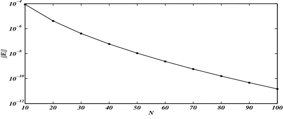
withθ(t) =qt,k(t, s) =ts, andg(t) = (−t2+t+ 1)et+t(qt−1)eqt, has the exact solutiony(t) =et_{. The results are shown in Table 1.}

Table 1: Values of∥E∥_∞for Example 1

N\q 0.01 0.09 0.1 0.5 0.99

10 3.7266×10−6 ₄_.₅₆₈₄_×₁₀−6 ₄_.₁₉₀₀_×₁₀−6 ₈_.₈₄₃₂_×₁₀−5 ₁_.₇₅₁₁_×₁₀−5

30 5.5006×10−10 ₃_.₆₁₄₈_×₁₀−9 ₅_.₂₄₅₀_×₁₀−9 ₄_.₀₉₄₆_×₁₀−7 ₇_.₅₅₃₀_×₁₀−8

50 8.6331×10−13 ₁_.₀₁₁₈_×₁₀−10 ₁_.₃₇₈₈_×₁₀−10 ₁_.₀₈₅₂_×₁₀−8 ₁_.₁₇₉₂_×₁₀−9

70 7.9936×10−15 ₅_.₄₁₅₂_×₁₀−12 ₇_.₃₆₈₃_×₁₀−12 ₅_.₈₁₅₃_×₁₀−10 ₁_.₀₆₈₈_×₁₀−10

90 3.2196×10−15 ₄_.₃₆₀₉_×₁₀−13 ₅_.₉₃₇₄_×₁₀−13 ₄_.₆₇₉₅_×₁₀−11 ₈_.₆₀₀₆_×₁₀−12

(11)

Galley

Pro

of

10 20 30 40 50 60 70 80 90 100

10−12 10−10 10−8 10−6 10−4

N

||E||

Figure 1: The errors forq= 0.5 in Example 1

y(t) =g(t) +

∫ tr

0

K(t, s)y(s)ds

withk(t, s) =s−t. We chooseg(t) so that its exact solution isy(t) =t−t2_. Table 2 shows the numerical results.

Table 2: Values of∥E∥_∞for Example 2

N\r 0.01 0.09 0.1 0.5 0.99

10 1.1098×10−6 ₄_.₆₃₇₃_×₁₀−6 ₅_.₃₄₁₈_×₁₀−6 ₅_.₂₆₈₆_×₁₀−6 ₅_.₅₇₉₆_×₁₀−6

30 4.0592×10−10 ₈_.₁₃₁₁_×₁₀−10 ₈_.₁₄₉₆_×₁₀−10 ₇_.₉₉₄₇_×₁₀−10 ₈_.₁₂₇₃_×₁₀−10

50 8.2652×10−13 ₁_.₃₆₃₁_×₁₀−12 ₁_.₄₀₂₇_×₁₀−12 ₁_.₃₂₈₉_×₁₀−12 ₁_.₃₈₉₈_×₁₀−12

70 4.8580×10−15 ₇_.₁₈₇₁_×₁₀−15 ₇_.₀₉₉₁_×₁₀−15 ₆_.₈₉₇₂_×₁₀−15 ₇_.₀₄₉₉_×₁₀−15

90 1.4498×10−16 ₂_.₂₇₀₆_×₁₀−16 ₁_.₉₄₂₈_×₁₀−16 ₁_.₆₆₅₃_×₁₀−16 ₃_.₃₃₀₆_×₁₀−16

10 20 30 40 50 60 70 80 90 100

10−16 10−14 10−12 10−10 10−8 10−6 10−4

N

||E||

(12)

Galley

Pro

of

8 Conclusion

Several methods has been presented for the numerical solution of equation (1) in the special cases for example θ(t) = qt[2]. We propose a numerical algorithm in order to solve the delay integral equation (Eq. (1)) where θ is general function. Our method has been shown theoretically and numerically to be extremely accurate and achieve exponential convergence with respect to N.

References

1. Brunner, H. Iterated collocation methods for Volterra integral equations with delay arguments, Math. Comput. 62 (1994), 581–599.

2. Brunner, H.,Collocation Methods for Volterra Integral and Related Func-tional Equations, Cambridge 2004.

3. Denisov, A.M. and Lorenzi, A. Existence results and regularisation tech-niques for severely ill-posed integrofunctional equations, Boll. Un. Mat. Ital. 11 (1997), 713–731.

4. Iserles, A.On the generalized pantograph functional differential equation, European J. Appl. Math. 4 (1993), 1–38.

5. Li, Y.K. and Kuang, Y.Periodic solutions of periodic delay Lotka-Volterra equations and systems, J. Math. Anal. Appl. 255 (2001), 260–280. 6. Linz, P. and Wang, R.L.C. Error bounds for the solution of Volterra and

delay equations, Appl. Numer. Math. 9 (1992), 201–207.

7. Okayama, T., Matsuo, T. and Sugihara, M.Error estimates with explicit constants for Sinc approximation, Sinc quadrature and Sinc indefinite in-tegration, Mathematical Engineering Technical Reports 2009-01, The Uni-versity of Tokyo, 2009.

8. Stenger, F. Handbook of Sinc Numerical Methods, Springer, New York 2011.

9. Stenger, F. Numerical Methods Based on Sinc and Analytic Functions, Springer, New York 1993.

10. Xie, H.H., Zhang, R. and Brunner, H.Collocation Methods for General Volterra Functional Integral Equations with Vanishing Delays, SIAM J. Sci. Comp. 33 (2011), 3303–3332.

(13)

یﺮﯿﺷ ﻼﯿﻟ و ﺎﯿﻧبرﺎﺿ ﺪﻤﺤﻣ

یدﺮﺑرﺎﮐ ﯽﺿﺎﯾر هوﺮﮔ ،ﯽﺿﺎﯾر مﻮﻠﻋ هﺪﮑﺸﻧاد ،ﯽﻠﯿﺑدرا ﻖﻘﺤﻣ هﺎﮕﺸﻧاد

١٣٩۴ ید ١٧ ﻪﻟﺎﻘﻣ شﺮﯾﺬﭘ ،١٣٩۴ رذآ ٢۵ هﺪﺷ حﻼﺻا ﻪﻟﺎﻘﻣ ﺖﻓﺎﯾرد ،١٣٩۴ ﺮﯿﺗ ٢ ﻪﻟﺎﻘﻣ ﺖﻓﺎﯾرد

ﺚﺤﺑ ﺮﯿﺧﺄﺗ ﻊﺑﺎﺗ ﺎﺑ اﺮﺘﻟو ﯽﻌﺑﺎﺗ لاﺮﮕﺘﻧا تﻻدﺎﻌﻣ ﻞﺣ یاﺮﺑ ﮏﻨﯿﺳ ﯽﻠﺤﻣ ﻢﻫ شور ،ﻪﻟﺎﻘﻣ ﻦﯾا رد : هﺪﯿﮑﭼ

شور ﻦﯾا .ﺖﺳا هﺪﺷ تﺎﺒﺛا تﻻدﺎﻌﻣ ﻦﯾا یاﺮﺑ ﯽﺒﯾﺮﻘﺗ یﺎﻫ باﻮﺟ ﯽﯾﺎﺘﮑﯾ و دﻮﺟو ﻦﯿﻨﭼ ﻢﻫ .ﺖﺳا هﺪﺷ ﯽﯾارﺎﮐ و ﺖﻗد ﺪﯿﯾﺄﺗ یاﺮﺑ یدﺪﻋ ﺞﯾﺎﺘﻧ .ﺪﻫد ﯽﻣ ﻪﺠﯿﺘﻧ ار ﯽﯾﺎﻤﻧ ﯽﯾاﺮﮕﻤﻫ و ﺪﺸﺨﺑ ﯽﻣ دﻮﺒﻬﺑ ار فرﺎﻌﺘﻣ ﺞﯾﺎﺘﻧ .ﺪﻧا هﺪﺷ ﻪﺋارا شور