The Student-t Mixture as a Natural Image Patch Prior
with Application to Image Compression
A¨aron van den Oord [email protected]
Benjamin Schrauwen [email protected]
Department of Electronics and Information Systems Ghent University
Sint-Pietersnieuwstraat 41, 9000 Ghent, Belgium
Editor:Ruslan Salakhutdinov
Abstract
Recent results have shown that Gaussian mixture models (GMMs) are remarkably good at density modeling of natural image patches, especially given their simplicity. In terms of log likelihood on real-valued data they are comparable with the best performing techniques published, easily outperforming more advanced ones, such as deep belief networks. They can be applied to various image processing tasks, such as image denoising, deblurring and inpainting, where they improve on other generic prior methods, such as sparse coding and field of experts. Based on this we propose the use of another, even richer mixture model based image prior: the Student-t mixture model (STM). We demonstrate that it convincingly surpasses GMMs in terms of log likelihood, achieving performance competitive with the state of the art in image patch modeling. We apply both the GMM and STM to the task of lossy and lossless image compression, and propose efficient coding schemes that can easily be extended to other unsupervised machine learning models. Finally, we show that the suggested techniques outperform JPEG, with results comparable to or better than JPEG 2000.
Keywords: image compression, mixture models, GMM, density modeling, unsupervised learning
1. Introduction
Recently, there has been a growing interest in generative models for unsupervised learning. Especially latent variable models such as sparse coding, energy-based learning and deep learning techniques have received a lot of attention (Wright et al., 2010; Bengio, 2009). The research in this domain was for some time largely stimulated by the success of the models for discriminative feature extraction and unsupervised pre-training (Erhan et al., 2010). Although some of these techniques were advertised as better generative models, no experimental results could support these claims (Theis et al., 2011). Furthermore recent work (Theis et al., 2011; Tang et al., 2013) showed that many of these models, such as restricted Boltzmann machines and deep belief networks are outperformed by more basic models such as the Gaussian Mixture model (GMM) in terms of log likelihood on real-valued data.
successful in various image processing tasks, such as denoising, deblurring and inpainting (Zoran and Weiss, 2011; Yu et al., 2012). Good density models are essential for these tasks, and the log likelihood measure of these models has shown to be a good proxy for their performance. Apart from being simple and efficient, GMMs are easily interpretable methods which allow us to learn more about the nature of images (Zoran and Weiss, 2012).
In this paper we suggest the use of a similar, simple model for modeling natural im-age patches: the Student-t mixture model (STM). The STM uses multivariate Student-t distributed components instead of normally distributed components. We will show that a Student-t distribution, although having only one additional variable (the number of degrees of freedom), is able to model stronger dependencies than solely the linear covariance of the normal distribution, resulting in a large increase in log likelihood. Although a GMM is a universal approximator for continuous densities (Titterington et al., 1985), we will see that the gap in performance between the STM and GMM remains substantial, as the number of components increases.
Apart from comparing these methods with other published techniques for natural image modeling in terms of log likelihood, we will also apply them to image compression by proposing efficient coding schemes based on these models. Like other traditional image processing applications, it is a challenging task to improve upon the well-established existing techniques. Especially in data compression, which is one of the older, more advanced branches of computer science, research has been going on for more than 30 years. Most modern image compression techniques are therefore largely the result of designing data-transformation techniques, such as as the discrete cosine transform (DCT) and the discrete wavelet transform (DWT), and combining them with advanced engineered entropy coding schemes (Wallace, 1991; Skodras et al., 2001).
We will demonstrate that simple unsupervised machine learning techniques such as the GMM and STM are able to perform quite well on image compression, compared with conventional techniques such as JPEG and JPEG 2000. Because we want to measure the density-modeling capabilities of these models, the amount of domain-specific knowledge induced in the proposed coding schemes is kept to a minimum. This also makes it relevant from a machine learning perspective as we can more easily apply the same ideas to other types of data such as audio, video, medical data, or more specific kinds of images, such as satellite, 3D and medical images.
In Section 2 we review some work on compression, in which related techniques were used. In Section 3 we give the necessary background for this paper on the GMM and STM and the expectation-maximization (EM) steps for training them. We will also elaborate on their differences and the more theoretical aspects of their ability to model the distribution of natural image patches. In Section 4 we present the steps for encoding/decoding images with the use of these mixture models for both lossy and lossless compression. The results and their discussion follow in Section 5. We conclude in Section 6.
2. Related Work
In this section we will review related work on image compression and density modeling.
2.1 Image Compression
The coding schemes (see section 4) we use to compare the GMM and STM, can be related with other published techniques in image compression, in the way they are designed. Al-though little research has been done on the subject we briefly review work based on vector quantization, sparse coding and subspace clustering. The lossy coding scheme we describe in this paper is based on a preliminary version that appeared in our previous work (van den Oord et al., 2013).
In vector quantization (VQ) literature, GMMs have been proposed for the modeling of low-dimensional speech signal parameters (Hedelin and Skoglund, 2000). In this setting, the GMMs’ probability density function is suggested to be used to fit a large codebook of VQ centroids on (e.g., with a technique similar to k-means), instead of on the original data set. They were introduced to help against overfitting, which is a common problem with the design of vector quantizers when the training set is relatively small compared to the size of the codebook. The same idea has also been suggested for image compres-sion (Aiyer et al., 2005). In contrast to these approaches we will apply a (learned) data transformation in combination with simple scalar uniform quantization, which reduces the complexity considerably given the relatively high dimensionality of image patches. This idea called transform coding (Goyal, 2001) is widely applied in most common image compression schemes, which use designed data-transforms such as the DCT and DWT.
By some authors (Hong et al., 2005) image compression has been suggested based on a subspace clustering model. The main contribution was a piecewise linear transformation for compression, which was also extended to a multiscale method. This is by some means similar to our lossy compression scheme as we also apply a piecewise linear transform, but based on the GMM/STM instead of a subspace clustering technique. They did not suggest quantization or entropy coding steps, and therefore only evaluated their approach in terms of energy compaction instead of rate-distortion.
Image compression based on sparse coding has been proposed (Horev et al., 2012) for images in general (Bryt and Elad, 2008; Zepeda et al., 2011) and for a specific class of facial images. Aside from being another unsupervised learning technique, sparse coding has been related with GMM in another way: Some authors (Yu et al., 2012; Zoran and Weiss, 2011) have suggested the interpretation of a GMM as a structured sparse coding model. This idea is based on the observation that data can often be represented well by one of the N Gaussian mixture components, thus when combining all the eigenvectors of their covariance matrices as an overcomplete dictionary, the sparsity is N1. The main results in Horev et al. (2012) show that sparse coding outperforms JPEG, but it does not reach JPEG 2000 performance for a general class of images.
2.2 Models of Image Patches
The Fields of Experts (FoE) framework is another approach for learning priors that can be used for image processing applications (Roth and Black, 2005; Weiss and Freeman, 2007). In a FoE, the linear filters of a Markov random field (MRF) are trained to maximize the log-likelihood of whole images in the training set. This optimization is done approximately with contrastive divergence, as computing the log likelihood itself is intractable. The po-tential functions that are used in the MRF are represented by a product of experts (PoE) (Hinton, 2002). The FoE is commonly used for image restoration tasks such as denoising and inpainting, but was also recently outperformed by GMMs with the expected patch log likelihood framework (EPLL) (Zoran and Weiss, 2012).
Recently similar models to the GMM have been proposed for image modeling, such as the Deep mixture of Factor analyzers (Deep MFA) (Tang et al., 2012). This technique is a deep generalization of the Mixture of Factor Analyzers model, which is similar to the GMM. The deep MFA has a tree structure in which every node is a factor analyzer, which inherits the low-dimensional latent factors from its parent.
Another model related to the GMM and STM is the Mixture of Gaussian scale mixtures (MoGSM) (Theis et al., 2011, 2012). Instead of a Gaussian, every mixture component is a Gaussian scale mixture distribution. The MoGSM has been used for learning multi-scale image representations, by modeling each level conditioned on the higher levels.
RNADE, a new deep density estimation technique for real valued data has a very dif-ferent structure (Uria et al., 2013b,a). RNADE is an extension of the NADE technique for real-valued data, where the likelihood function is factored into a product of conditional likelihood functions. Each conditional distribution is fitted with a neural mixture density network, where one variable is estimated, given the other ones. Recently a new training method has allowed a factorial number of RNADE’s to be trained at once within one model. It is currently one of the few deep learning methods with good density estimation results on real-valued data and is the current state of the art on image patch modeling.
3. Mixture Models as Image Patch Priors
Mixture models are among the most widely accepted methods for clustering and probability density estimation. Especially GMMs are well known and have widespread applications in different domains. However depending on the data used, other mixture models might be more suitable.
In this work we will denote the mixture component distribution as fk and the mixture
distribution as
f(x) =
K
X
k=1
πkfk(x),
where πk, k = 1. . . K are the mixing weights. The two component distributions we study
here are the multivariate normal distribution:
fk(x) =N(x|µk,Σk) = (2π)−
p
2|Σk|− 1 2 e−
1 2(x−µk)
TΣ−1
k (x−µk),
and the multivariate Student-t distribution, see Equation 1. In these equations, p is the dimensionality ofx. We will train the GMM with the EM-algorithm: an iterative algorithm
for finding the maximum likelihood estimate of the parameters. For completeness we sum-marize the expectation and maximization steps for training a GMM with EM.
E-step:
γnk =
πkN (xn|µk,Σk) K
P
j=1
πjN(xn|µj,Σj)
.
M-step:
πk=
1
N
N
X
n=1
γnk, µk=
N
P
n=1 γnkxn
N
P
n=1 γnk
,
Σk = N
P
n=1
γnk(xn−µk) (xn−µk)T
N
P
n=1 γnk
.
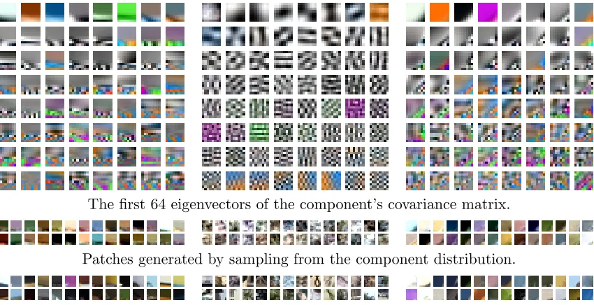
One of the important reasons GMMs excel at modeling image patches is that the distri-bution of image patches has a multimodal landscape. A unimodal distridistri-bution such as the multivariate normal distribution is not able to capture this. When using a mixture however, each component can represent a different aspect or texture of the whole distribution. We can observe this by looking at the individual mixture components of a trained GMM model, see Figure 1.
Next to modeling different textures, the GMM also captures differences in contrast. It has been shown (Zoran and Weiss, 2012) that multiple components in the GMM describe a similar structure in the image, but each with a different level of contrast. The STM, however, can model different ratios of contrast within a single mixture component.
A multivariate Student-t distribution has the following density function (Kotz and Nadarajah, 2004):
T (x|ν, µ,Σ) = Γ
ν+p
2
Γ ν2
νp2π
p
2 |Σ|1/2
1 + 1
ν (x−µ) T
Σ−1(x−µ)
−ν+2p
. (1)
ν is an additional parameter which represents the number of degrees of freedom. Note that forν→ ∞the Student-t distribution converges to the normal distribution. It is interesting to see how this distribution is constructed:
If Y is a multivariate normal random vector with mean 0 and covariance Σ, and if νT is a chi-squared random variable with degrees of freedom ν, independent of Y, and
X= √Y
T +µ,
The first 64 eigenvectors of the component’s covariance matrix.
Patches generated by sampling from the component distribution.
Examples from the train set that are best represented by this component.
The first 64 eigenvectors of the component’s covariance matrix.
Patches generated by sampling from the component distribution.
Examples from the train set that are best represented by this component.
variety of contrast, for a given texture. The distribution ofT is visualized in Figure 2(a), for different values ofν. If ν is small for a given component (texture), this means that the texture appears in natural images in a wide range of contrast. Forν→ ∞we get a Gaussian distribution and its contrast is more constrained. To obtain the same capacity with a GMM, one would need multiple components having scaled versions of the same covariance matrix. In Figure 2(b) the value of ν is visualized for different components of a trained STM. This value differs substantially for each component, ranging from almost zero to 15. This means some component-distributions are very long-tailed (with smallν) and some are more normally distributed (higher ν). This means that some texture patterns appear in a wider range of contrast than others. However, in our experiments we saw that the STM does not learn significantly different structures compared to the GMM. The texture patterns learned by the STM were also very similar to those shown in Figure 1. This means the STM is better at generalizing to image patches with different levels of contrast, but might not be better at generalizing to different unseen texture patterns.
0.0 0.5 1.0 1.5 2.0 2.5 3.0 0.0
0.5 1.0 1.5 2.0 2.5 3.0
ν = 1 ν = 3 ν = 10 ν = 100
(a) The distribution ofT in Equation 2, for different
values ofν. Asν increases the distribution becomes
more peaked and converges to a Dirac delta at 1.
0 20 40 60 80 100 120 140 0
2 4 6 8 10 12 14 16
νk
(b) The value ofνkfor each componentkof a trained
STM with 128 components, sorted from low to high.
Figure 2: The distribution of T for different ν and the value of ν for different mixture components.
with more mixture components the risk of overfitting also increases. If one would tie the parameters of some of these components together, so that they have scaled versions of the same covariance matrix, the risk of overfitting would decrease. This is exploited in the mixture of Gaussian scale mixtures (MoGSM) (Theis et al., 2012).
The idea of explicitly sharing covariance parameters between mixture components has also been applied to mixtures of factor analyzers, with the deep MFA model (Tang et al., 2012). They proposed a hierarchical structure in which the mixture components partially inherit the covariance structure of their parent in the hierarchy.
The Student-t has previously been used for modeling image patches in the PoE frame-work (Welling et al., 2002), where each expert models a differently linearly filtered version of the input with a univariate Student-t distribution.
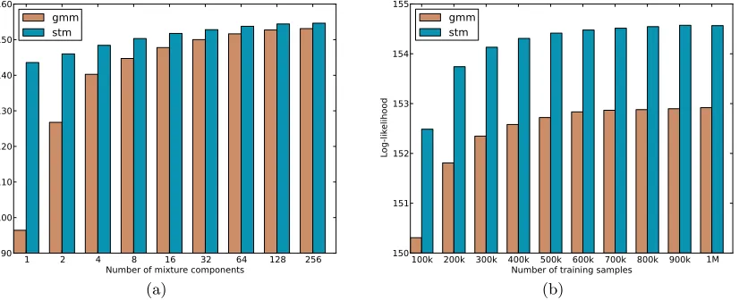
1 2 4 8 16 32 64 128 256
Number of mixture components 90 100 110 120 130 140 150 160 Lo g-l ike lih oo d gmm stm (a)
100k 200k 300k 400k 500k 600k 700k 800k 900k 1M Number of training samples
150 151 152 153 154 155 Lo g-l ike lih oo d gmm stm (b)
Figure 3: The average patch log likelihood for the Gaussian mixture model (GMM) and Student-t mixture model (STM) in function of its number of mixture compo-nents (a) and number of training samples (b). The models were trained on 8x8 normalized gray scale image patches, extracted from the Berkeley data set (see Section 5.1.1).
We also train the STM with the EM algorithm (Peel and McLachlan, 2000; Dempster et al., 1977):
E-step:
γnk =
πkT (xn|νk, µk,Σk) K
P
j=1
πjT (xn|νj, µj,Σj)
, wnk = ν νk+p
k+(xn−µk)TΣk−1(xn−µk) .
M-step:
πk=
1
N
N
X
n=1
γnk, µk=
N
P
n=1
γnkwnkxn
N
P
n=1 γnkwnk
.
Σk= N
P
n=1
γnkwnk(xn−µk) (xn−µk)T
N
P
n=1 γnk
.
For the degrees of freedom, there is no closed form update rule. Instead νkgets updated as
the solution of:
−ψνk
2
+ logνk 2
+ 1 + 1
αk N
X
n=1
γnk(log (wnk)−wnk)
+ψ
˜
νk+p
2
−log
˜
νk+p
2
= 0,
where ˜νk is the value of the current νk, αk =
PN
n=1γnk and ψ is the digamma function.
This scalar non-linear equation can be solved quickly with a root finding algorithm, such as Brent’s method (Brent, 1973).
Note that the expectation and maximization steps are quite similar to those of the GMM. In our experiments, it did not take substantially longer to train a STM than a GMM. Typically 100 iterations were enough to train the STM or GMM, even though the log likelihood does keep improving a little bit after that (even after 500 iterations). For a big mixture model of 256 components, trained on 500.000 samples of 8x8 gray scale patches, this took about 20 hours on a standard desktop computer with four cores. For the STM, it took 21 hours. On this scale, the CPU time is linear in both the number of training samples and the number of components. Training on image patches proved to be quite stable: no components needed to be reinitialized during training.
The code for training a Student-t mixture is included in the supplementary material of this paper.
4. Compression with Mixture Models
Both the lossy and lossless algorithms we propose are patch/block based. This means they will encode each patch of an image separately. During training we randomly sample a large set of image patches from the training images. These are used to fit the GMM and STM models. Once training is finished, these density models can be used to encode the test images. Each test image is viewed as a grid of non-overlapping patches. The encoder loops over all patches, which are extracted, flattened and encoded one by one.
To speed up the algorithms, each patch will be encoded using the distribution and parameters of only one of the mixture components. We choose the mixture component which represents the given patch with the highest likelihood:
β = arg max
k fk(xn).
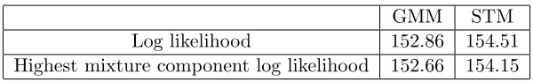
GMM STM
Log likelihood 152.86 154.51
Highest mixture component log likelihood 152.66 154.15
Table 1: Average patch log likelihood compared with the average highest component patch log likelihood: How well can a sample be represented by using a single mixture component? (See text)
on a validation set. We have also computed the average log likelihood when only one of the mixture components is used for each example: N1 PN
n=1log (maxk(πkfk(xn))). Note that
this is strictly lower than the actual average log likelihood: N1 PN
n=1log
PK
k=1πkfk(xn)
. But as can be seen from Table 1, the difference is small.
4.1 Arithmetic Coding
Most commonplace image compression schemes follow three main steps: transformation, quantization and entropy coding (Goyal, 2001). Transformation decorrelates the data, quan-tization maps the values of the decorrelated continuous variables onto discrete values from a relatively small set of symbols (such as integers) and entropy coding encodes these discrete quantized values into a bit sequence. In this paper, transformation and quantization will only be used for lossy compression and not for lossless compression. However, in both cases we employ arithmetic coding (AC) for the entropy coding step.
Entropy coding is a family of algorithms that take as input a sequence of discrete values, and give as output the encoded binary sequence. Based on the statistical properties of the input, the goal is to minimize the expected length of the bit sequence (e.g., by assigning more bits to a rare symbol and less bits to a common symbol). The theoretical limit of the encoding scheme is bounded by the entropy of the input signal, which explains the name entropy coding. Arithmetic coding is a form of entropy coding, which requires a list of probabilities αi, i = 1. . . N that describe the discrete distribution P(sj) = αj of
a symbol sj occurring in an input sequence. Based on these probabilities, the algorithm
will on average spend fewer bits on common symbols, than on rare ones. However, with AC it is also possible to use different probabilities for each time step t in the sequence:
P
s(jt)
=αjt, and even adapt them during the encoding/decoding based on the values of
the previously encoded symbols. This is also called adaptive arithmetic coding.
4.2 Lossless Compression
In lossless compression, the image should be preserved perfectly so that after decompression the output image is identical to the input image. Because we have a probabilistic model for an image patch, the most natural way to approach this task is to use lossless predictive coding (Pearlman and Said, 2011). The idea is to predict the value (integer) of each sample within an image patch, using the values of its neighboring samples that are already encoded, based on the correlations between them. In this case, the prediction will actually consist of
a discrete probability distribution over the possible values of the current sample, which can directly be used to perform arithmetic coding.
To carry out arithmetic coding on a patchxi, one needs to compute a list of probabilities
(probability table) for each of its elementsxi,j: P(xi,j =l) forl= 0. . . L. More specifically,
because arithmetic coding can adapt the probability tables to the information of the previous symbolsxi,1. . . xi,j−1 it is possible to encode every symbol conditionally with respect to the
ones already encoded: P(xi,j = l|xi,1. . . xi,j−1). As the image patches are modeled by
continuous probability densities, this can computed as follows:
P(xi,j =l|xi,1. . . xi,j−1) = Z l+1
2
l−1 2
f(xi,j|xi,1. . . xi,j−1) dxi,j. (2)
This scheme for performing lossless image compression can be used in combination with any density model, provided that we can compute Equation 2. This way arithmetic coding can be applied to the image using the statistics of the trained model. Algorithm 1 gives a summary for lossless compression with a mixture model.
As already mentioned, when using an mixture model, it is more efficient to use a single component for the encoding of a patch than the whole mixture. For both normally and Student-t distributed variables, the expressions for Equation 2 can be derived from their conditional distributions.
For the normal distribution this becomes:
Z l+1
2
l−1 2
N(xi,j|xi,1. . . xi,j−1) dxi,j =Fn
l+1
2|µ˜j,σ˜j
2
−Fn
l−1
2|µ˜j,σ˜j
2
,
withFn the cumulative distribution function (CDF) of the univariate normal distribution,
and where
˜
µj =µj+ Σj,1:j−1Σ−1:1j−1,1:j−1(x1:j−1−µ1:j−1),
˜
σj2 = Σj,j−Σj,1:j−1Σ1:−1j−1,1:j−1Σ1:j−1,j.
For the multivariate Student-t distribution the equations are similar:
Z l+12
l−1 2
T (xi,j|xi,1. . . xi,j−1) dxi,j =Ft
l+1
2|ν˜j,µ˜j,s˜j
2
−Ft
l− 1
2|ν˜j,µ˜j,s˜j
2
,
with Fn the CDF of the non-standardized univariate Student-t distribution (which has a
location and scale parameter), and where
˜
νj =νj+j−1,
˜
µj =µj+ Σj,1:j−1Σ−1:1j−1,1:j−1(x1:j−1−µ1:j−1),
˜
sj2=
ν+xT1:j−1Σ1:−j1−1,1:j−1x1:j−1 ν+j−1
!
Σj,j−Σj,1:j−1Σ1:−j1−1,1:j−1Σ1:j−1,j
.
When using a form of entropy coding, such as arithmetic coding, the theoretical optimal code length for a symbol i is dependent on the probability Pi of it occurring: −log (Pi).
Therefore, the lower bound on the expected rate (bits per symbol) is: −1
N
PN
i=1Pilog (Pi).
Because Pi is calculated by a density model (Equation 2), the log likelihood score of this
Algorithm 1: Lossless image compression with a mixture model. [AC] stands for arithmetic coding.
Encoder:
for each patch xi in image do
β= arg maxkfk(xi)
[AC] Encode symbolβ with probability table π (mixing weights) foreach xij, j= 1. . . p do
Use Equation 2 to compute: αi,j,l=Pβ(xi,j =l|zi,1. . . xi,j−1)
[AC] Encode symbolxij with probability tableαi,j
end end
Decoder:
while not at end of bit stream do
[AC] Decode symbolβ with probability table π (mixing weights) initializexi
forj= 1. . . p do
Use Equation 2 to compute: αi,j,l=Pβ(xi,j =l|zi,1. . . xi,j−1)
[AC] Decode symbolxij with probability table αi,j
end end
Reconstruct image from patches xi, i= 1. . . N.
4.3 Lossy Compression
For lossy compression, the image reconstruction after decompression does not have to be identical to the original, but should match it very closely. The strength of compression should be as high as possible, given a certain tolerable amount of distortion. This freedom evidently allows stronger compression than with lossless algorithms.
Lossy image compression algorithms typically use quantization to reduce the amount of information that needs to be entropy coded. Quantization decreases the number of states of the data variables to a smaller discrete set. As mentioned above we will use simple scalar quantization as the number of variables in a patch is relatively high and vector quantization would simply be impractical. Instead of VQ, we will combine scalar quantization with a data transform step, as is done in most image compression schemes.
The main reason of a data transform step in compression schemes is to decorrelate the input, so that the different coefficients can be handled more independently afterwards. Es-pecially when using scalar quantization it is important to use a form of transformation first, as this reduces the amount of redundancy in the data that has to be encoded. Moreover, if one would quantize the image in the original pixel domain, the reconstruction artifacts would be very obtrusive. Because a Gaussian or Student-t mixture component already models covariance, decorrelation is fairly straightforward. The transform step is as follows:
yi =WT(xi−µ), (3)
where W is the eigenvector matrix of the covariance matrix Σ of the Gaussian/Student-t mixture component: W J WT = Σ. J is the diagonal eigenvalue matrix of Σ. Subsequently, the transformed values are quantized with a uniform quantizer:
zi = round
yi λ
. (4)
The strength of the quantization only depends on λ. When it is high, the quality of the encoded image will be low, but the compression ratio will be high.
Once quantization is done, arithmetic coding is carried out in a similar fashion as with lossless compression: we have to be able to compute Equation 2. Because the data is transformed (Equation 3), the mean of y becomes 0: µy = 0 and the covariance matrix
reduces to: Σy =J. The equations for calculating the conditional probabilities from before
can now be simplified. For the normal distribution:
P(zi,j=l|zi,1, . . . , zi,j−1) =
Z λ(l+1
2)
λ(l−1 2)
N(yi,j|y˜i,1. . .y˜i,j−1) dyi,j (5)
= Fn
λ
l+1
2
|0, Jj
−Fn
λ
l−1
2
|0, Jj
,
withFn the cumulative distribution function (CDF) of the univariate normal distribution,
For the Student-t distribution:
P(zi,j =l|zi,1, . . . , zi,j−1) =
Z λ(l+1
2)
λ(l−1 2)
T (yi,j|y˜i,1. . .y˜i,j−1) dyi,j (6)
= Ft
λ
l+1
2
|ν˜j,0,s˜j2
−Ft
λ
l−1
2
|ν˜j,0,s˜j2
,
with Ft the CDF of the non-standardized univariate Student-t distribution (which has a
location and scale parameter), and where
˜
νj =νj+j−1,
˜
sj =
νj +Pjm−=11
˜
y2
i,m
Jm νj +j−1
Jj.
Because of the two additional steps (Transformation and Quantization) during compres-sion, the decoder has to dequantize and subsequently detransform the data after arithmetic coding.
Dequantization:
˜
yi =λzi. (7)
Inverse transform:
˜
xi=Wy˜i+µ. (8)
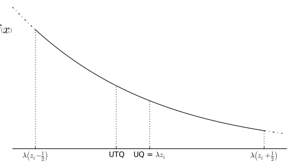
4.3.1 Uniform Threshold Quantization
It is important to note that Equation 7 might not be the best choice for reconstruction. It is indeed possible to increase the quality of dequantization by using prior knowledge of the scalar input distribution. This concept is called uniform threshold quantization (Pearlman and Said, 2011). Figure 4 shows the difference with regular uniform quantization.
Depending on the assumed distribution of the source it is possible to minimize the expected distortion: (˜yi,j−yi,j)2 (other measures of distortion can also be used). This
comes down to solving the following optimization problem:
˜
yi,j = arg min y
Z λ(zi,j+1
2)
λ(zi,j−12)
ky−xk2f(x) dx,
which can be simplified to:
˜
yi,j =
Rλ(zi,j+12)
λ(zi,j−12) xf(x) dx
Rλ(zi,j+12)
λ(zi,j−12) f(x) dx .
This is actually nothing more than the centroid in that region (see Figure 4). Because we are using a probabilistic method, this improved reconstruction almost comes for free: The
Algorithm 2:Lossy image compression with a mixture model. [AC] stands for arith-metic coding.
Encoder:
for each patch xi in image do
β= arg maxkfk(xi)
[AC] Encode symbolβ with probability table π (mixing weights) Transformxi with Equation 3 using theβ-th component
Quantizexi with Equation 4
foreach xij, j= 1. . . p do
Use Equation 5 or 6 to compute: αi,j,l =Pβ(xi,j =l|xi,1. . . xi,j−1)
[AC] Encode symbolxij with probability tableαi,j
end end
Decoder:
while not at end of bitstream do
[AC] Decode symbolβ with probability table π (mixing weights) initializexi
forj= 1. . . p do
Use Equation 5 or 6 to compute: αi,j,l =Pβ(xi,j =l|xi,1. . . xi,j−1)
[AC] Decode symbolxij with probability table αi,j
end
Dequantizexi with Equation 7 or 9
Inverse transformxi with Equation 8
end
λzi−12 λ
zi+12
UQ = λzi
UTQ
f
(x
)Figure 4: Uniform quantization versus uniform threshold quantization. During dequantiza-tion, UQ will reconstruct the input with the centers of the quantization intervals. UTQ uses the centroids instead.
compression scheme remains the same, only the decompression is improved. For a normally distributed variable the reconstruction is
˜
yi,j =
q Jj 2π exp −λ
2(z
i,j−12)
2
2Jj
−exp
−λ
2(z
i,j+12)
2
2Jj
Fn λ zi,j+12
|0, Jj
−Fn λ zi,j −12
|0, Jj
,
and for a Student-t distributed variable it is
˜
yi,j=
Γνj˜2+1 √
πΓνj˜2 ˜
sνjj˜ν˜j
˜
νj
2
˜
νj−1
"
˜
νj˜s2j+λ2 zi,j−12
2 1−νj˜
2
−ν˜js˜2j+λ2 zi,j+12
2 1−νj˜
2 #
Ft λ zi,j+12|ν˜j,0,s˜j2−Ft λ zi,j−12|ν˜j,0,s˜j2
.
5. Results and Discussion
In this section we will discuss the experimental results of the STM on density modelling and image compression tasks.
5.1 Data Sets and Methods
We will first introduce the data sets that we used for our experiments and also discuss the image compression standards (JPEG, JPEG 2000) which will be used to compare the compression results with.
5.1.1 Berkeley Segmentation Data Set
The Berkeley Segmentation Data set (Martin et al., 2001) consists of 200 training and 100 test JPEG-encoded images, originally intended to be used as a segmentation benchmark.
Some samples can be seen on Figure 5. This data set has been used by several authors to measure the unsupervised learning performance of their model on image patches (Zoran and Weiss, 2011; Tang et al., 2013; Uria et al., 2013a). We adopt the use of this data set for measuring density modeling performance, but not for image compression, as these images were already encoded with JPEG and will already contain some quantization noise.
5.1.2 UCID Data Set
Although images are abundant on the world wide web, large data sets containing losslessly encoded images are rather hard to find. In image processing most authors have grown to rely on a particular set of standard images, such as Lena, Baboon, Peppers, etc. 1 to measure
their algorithms’ performance. Although each of these images have specific features that make them interesting to test a new method on, results on this small set likely will not generalize to a wide range of images. Furthermore, because there is no clear distinction between a training and test set for these images, there is a high risk of overfitting (even when engineering a compression scheme). Finally most of these images are relatively old and noisy, so they are hardly representative for images of modern photography.
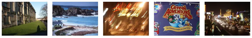
On of the few publicly available data sets is UCID (Schaefer and Stich, 2003) (Uncom-pressed Colour Image Data set). The UCID database consists of 1338 TIFF images on a variety of topics including natural scenes and man-made objects, both indoors and out-doors. The camera settings were all set to automatic as this resembles what the average user would do. All the images have sizes 512x384 or 384x512. The images are in true color (24-bit RGB, each color channel having 256 possible values per pixel). Some sample UCID images can be seen on Figure 6.
As the images are not in random order, we have included every 10th image (10, 20, 30,
. . ., 1330) of the data set in our test set, and the others were used for training. This results in 1205 images for training and 133 images for testing. We randomly sample a large set of image patches (two million) for training the mixture models. We then encode every test image with a number of different quantization strengths (only for lossy compression), and measure their compression performance and the distortion of their reconstruction.
5.1.3 JPEG and JPEG 2000
For comparison we added two image compression standards as benchmark: JPEG (Wallace, 1991) and JPEG 2000 (Skodras et al., 2001).
JPEG is a patch based compression standard which uses the DCT as its transform, with quantization and entropy coding optimized for this transform. For the JPEG standard, we employed the widely used libjpeg implementation (ijg.org). Optimization of the JPEG entropy encoding parameters was enabled for better performance. The quality parameter was swept from 0 (worst) to 100 (best) in steps of 5.
JPEG 2000 is a wavelet-based compression standard and because of its multiresolution decomposition structure, it is able to exploit wider spatial correlations than JPEG and our method (which are patch based). For JPEG 2000, the kakadu implementation was
1. Most of these standard images can be found here: http://sipi.usc.edu/database/database.php?
used (kakadusoftware.com). To make a fair comparison, command line parameters were enabled to optimize the PSNR instead of perceptual error measures.
For both methods we did not take the meta information of the header into account when measuring the performance of compression.
Figure 5: Sample images from the Berkeley Segmentation Data set.
Figure 6: Sample images from the UCID data set (Uncompressed Colour Image Data set).
5.2 Average Patch Log Likelihood Comparison
Two million 8x8 patches were extracted from the training images, and 50,000 were extracted from the testing images (Berkeley data set). For every sample the mean was subtracted (DC component). Because the test patches we extracted could differ from those used by other authors, we report the mean and standard deviation across 10 randomly sampled sets of 50,000 patches. The results are listed in Table 2. The GMM and STM had 200 mixture components. As expected our GMM has a comparable result to that reported in literature. The proposed method STM significantly outperforms other methods.
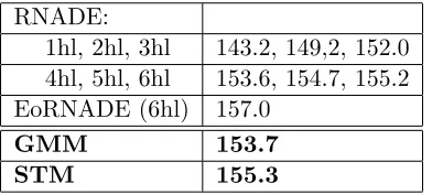
We also compare our result with the recently proposed RNADE model (Uria et al., 2013b,a). Because the authors preprocess the gray scale patches differently, the results are not comparable to the ones reported in Table 2. Before subtracting the sample mean, small uniform noise (between 0 and 1) is added to the pixel values (between 0 and 255), which are then normalized by dividing by 256. Afterwards, they remove the last pixel, so that the number of variables of each datapoint equals 63. For this task we used four million patches during training and evaluated on one million patches from the test set. The results are shown in Table 3. The STM outperforms the deep RNADE model of 6 layers, but is on its turn outperformed by the ensemble of RNADE models (EoRNADE).
5.3 Lossless Compression
Because JPEG does not natively support lossless compression we excluded this benchmark for this test. For our methods we used patch size 8x8 and 128 mixture components. The results are listed in Table 4. As explained above (see Section 4.2), there is a connection
Indp. Pixel ICA GRBM DBN MFA
78.3 135.7 137.8 144.4 166.5
Deep MFA MTA GMM GMM STM
169.3 158.2 167.2 166.97 ± 0.36 172.13 ± 0.42
Table 2: Average log-likelihood (higher is better). Own results are marked in bold. The results of other methods are taken from Zoran and Weiss (2011); Tang et al. (2013). ICA: independent component analysis, GRBM: Gaussian restricted Boltzmann machine, DBN: Deep belief network, MFA: mixture of factor analyzers, MTA: Mixture of Tensor analyzers.
RNADE:
1hl, 2hl, 3hl 143.2, 149,2, 152.0 4hl, 5hl, 6hl 153.6, 154.7, 155.2 EoRNADE (6hl) 157.0
GMM 153.7
STM 155.3
Table 3: Average log-likelihood comparison with RNADE (Uria et al., 2013a) in function of the number of hidden layers (hl). Our results are marked in bold. These results are obtained from differently processed patches than those in Table 2 (see text). EoRNADE stands for an ensemble of RNADE’s.
between average log likelihood and the expected lossless compression strength. The STM also outperforms the GMM on this task, and both methods outperform JPEG 2000.
5.4 Lossy Compression
We will first analyze the influence of the patch size on the lossy compression performance. The results are visualized in Figure 7. All mixture models were trained for 500 iterations and consist of 128 components. The reconstruction quality of an image is measured in peak signal-to-noise ratio: PSNR = 10 log10MSER2 , with R being the largest possible pixel value (255 in this case) and MSE being the average mean squared error.
Bigger patch sizes show better results for low bit rates and vice versa. This can be explained by the fact that when using larger patch sizes, covariance between more pixels
JPEG 2000 GMM STM
12.40 12.07 11.83
can be modeled simultaneously. This way the transform has the ability to decorrelate better, which is important for low bit rates. For higher bit rates, we approach a near-lossless region, where the log likelihood performance of the model is crucial. When modeling smaller patch sizes, the algorithm is less prone to overfit, resulting in better performance. We can see that these high-rate effects are most apparent for the GMM. The STM, which is more robust to overfitting, is able to model larger patch sizes.
Because the 8x8 patch size has a good performance in general for both methods, our final experiments are computed with this setting. Note that JPEG also uses 8x8 patches for its compression scheme. For different compression strengths we have computed the average PSNR of the reconstructed images. For some images, JPEG or JPEG 2000 was unable to encode them at a given rate (1, 2 and 10 images for 3, 4 and 5 bpp respectively), so these images where not taken into account at those rates.
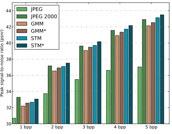
The final results are shown on Figure 8. For all compression rates, JPEG is outperformed by the other methods. The proposed compression schemes are competitive with JPEG 2000, and relatively to JPEG they score quite similar. In all experiments uniform threshold quantization improves on standard uniform quantization. The GMM is always outperformed by the STM, and the difference increases for larger bit rates. JPEG 2000 slightly exceeds the performance of the GMM in all experiments, but is in turn surpassed by the STM, with the exception of the lowest bit rate. At low bit rates, correlations on a more global scale become more important, which is why the multiresolution wavelet transform of JPEG 2000 achieves a better performance than our patch-based approach in this setting. Extending our approach to a multiscale technique might therefore be a promising direction of future research.
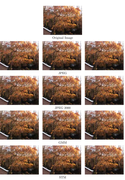
In Figure 9 we have visualized some reconstructed images after compression with JPEG, JPEG 2000 and the proposed method (GMM and STM), for varying levels of compression strength: 1, 2.5 and 5 bits per pixel (bpp). This Figure is best viewed on the electronic version by zooming in on the different images. Because JPEG and the proposed method are block based, they have blocking artifacts that JPEG 2000 does not. The latter has more blurring artifacts. The proposed method seems to have the strongest visual artifacts in low-frequency regions, but performs well in high-frequency regions such as trees and leaves. This can be attributed to the fact that the compression method does not take into account the properties of human visual perception and therefore quantizes both high as low frequency regions equally strongly. One could improve the visual results by adding prior knowledge about the perceptual system, using a deblocking filter (or using an image reconstruction algorithm based on GMM/STMs with the expected patch log likelihood (EPLL) framework), extending the model so that it works with overlapping blocks (with the MDCT transform for example) or by making it multi-scale. However, these extensions are outside the scope of this work.
6. Conclusion and Future Work
The presented work consists of two main contributions: the introduction and analysis of the Student-t mixture as an image patch modeling technique, and the proposal of lossless and lossy image compression techniques based on mixture models.
0 1 2 3 4 5 6 7
bits per pixel (bpp)
25 30 35 40 45 Pe ak si gn al -t o-no ise r at io ( psn r) GMM 4x4 GMM 6x6 GMM 8x8 GMM 10x10 GMM 12x12
0 1 2 3 4 5 6 7
bits per pixel (bpp)
25 30 35 40 45 Pe ak si gn al -t o-no ise r at io ( psn r) STM 4x4 STM 6x6 STM 8x8 STM 10x10 STM 12x12
Figure 7: Average patch Quality (PSNR) - Rate (bpp) curves for different patch-sizes (GMM left, STM right). This Figure is best viewed in color.
1 bpp 2 bpp 3 bpp 4 bpp 5 bpp
30 32 34 36 38 40 42 44 Pe ak si gn al -t o-no ise r at io ( psn r) JPEG JPEG 2000 GMM GMM* STM STM*
In the first part we have proposed the STM as an image patch prior. This method significantly outperformed the GMM for density modeling of image patches, with results competitive to the state-of-the-art on this task. This performance could largely be at-tributed to the fact that a Student-t mixture is able to model contrast in addition to linear dependencies within a single mixture component. For future work it would also be very interesting to see how it matches up with other methods on other types of data. Another possibility would be to study the Student-t mixture model for the use of image reconstruc-tion applicareconstruc-tions (denoising, deblurring, inpainting), as was recently proposed with GMMs (Zoran and Weiss, 2011).
In the second part both the GMM and STM have been examined in this paper for the task of image compression. Lossless and lossy coding schemes were presented, which could easily be adapted for other unsupervised learning techniques. For lossy compression, experimental results demonstrated that the proposed techniques consistently outperform JPEG, with results similar to those of JPEG 2000. With the exception of the lowest bit rate, the STM has the advantage over JPEG 2000 in terms of rate-distortion. In lossless compression both the GMM and STM outperform JPEG 2000, which is mainly due to the fact that this task is even more connected with density estimation. In future work, even more advanced techniques will be considered. Moving beyond the 8x8 patch size, with for example multiscale techniques, is an especially promising direction.
One of the most important conclusions we can draw here is that relatively simple machine learning techniques can perform quite well on the task of image compression. We saw that their performance could largely be attributed to their density modeling capabilities. It would therefore be interesting to apply machine learning to compression of different types of data, such as audio, video, EEG, etc. and more specific types of data such as facial or satellite images. We also propose for compression to be used more in machine learning as a benchmark to compare models. Given the recent progress in unsupervised machine learning we expect that even better results will follow.
References
Anuradha Aiyer, Kyungsuk Pyun, Ying-zong Huang, Deirdre B OBrien, and Robert M Gray. Lloyd clustering of Gauss mixture models for image compression and classification. Signal Processing: Image Communication, 20(5):459–485, 2005.
Yoshua Bengio. Learning deep architectures for AI. Foundations and TrendsR in Machine Learning, 2(1):1–127, 2009.
Richard P Brent. Algorithms for Minimization without Derivatives. Courier Dover Publi-cations, 1973.
Ori Bryt and Michael Elad. Compression of facial images using the k-svd algorithm.Journal of Visual Communication and Image Representation, 19(4):270–282, 2008.
Arthur P Dempster, Nan M Laird, and Donald B Rubin. Maximum likelihood from in-complete data via the em algorithm. Journal of the Royal Statistical Society. Series B (Methodological), pages 1–38, 1977.
Original Image
JPEG
JPEG 2000
GMM
STM
Michael Elad and Michal Aharon. Image denoising via sparse and redundant representations over learned dictionaries. Transactions on Image Processing, 15(12):3736–3745, 2006.
Dumitru Erhan, Yoshua Bengio, Aaron Courville, Pierre-Antoine Manzagol, Pascal Vincent, and Samy Bengio. Why does unsupervised pre-training help deep learning? The Journal of Machine Learning Research, 11:625–660, 2010.
Vivek K Goyal. Theoretical foundations of transform coding. Signal Processing Magazine, 18(5):9–21, 2001.
Per Hedelin and Jan Skoglund. Vector quantization based on Gaussian mixture models. Transactions on Speech and Audio Processing, 8(4):385–401, 2000.
Geoffrey E Hinton. Training products of experts by minimizing contrastive divergence. Neural Computation, 14(8):1771–1800, 2002.
Wei Hong, John Wright, Kun Huang, and Yi Ma. A multiscale hybrid linear model for lossy image representation. InInternational Conference on Computer Vision, volume 1, pages 764–771. IEEE, 2005.
Inbal Horev, Ori Bryt, and Ron Rubinstein. Adaptive image compression using sparse dictionaries. In International Conference on Systems, Signals and Image Processing, pages 592–595. IEEE, 2012.
Samuel Kotz and Saralees Nadarajah. Multivariate t-Distributions and their Applications. Cambridge University Press, 2004.
Julien Mairal, Francis Bach, Jean Ponce, Guillermo Sapiro, and Andrew Zisserman. Non-local sparse models for image restoration. In International Conference on Computer Vision, pages 2272–2279. IEEE, 2009.
David Martin, Charless Fowlkes, Doron Tal, and Jitendra Malik. A database of human segmented natural images and its application to evaluating segmentation algorithms and measuring ecological statistics. In International Conference on Computer Vision, vol-ume 2, pages 416–423, July 2001.
Bruno A Olshausen and David J Field. Sparse coding with an overcomplete basis set: A strategy employed by v1? Vision Research, 37(23):3311–3325, 1997.
William A Pearlman and Amir Said. Digital Signal Compression: Principles and Practice. Cambridge University Press, 2011.
David Peel and Geoffrey J McLachlan. Robust mixture modelling using the t distribution. Statistics and Computing, 10(4):339–348, 2000.
Stefan Roth and Michael J Black. Fields of experts: A framework for learning image priors.
In Computer Vision and Pattern Recognition, 2005., volume 2, pages 860–867. IEEE,
2005.
Gerald Schaefer and Michal Stich. UCID: an uncompressed color image database. In Electronic Imaging 2004, pages 472–480. International Society for Optics and Photonics, 2003.
Athanassios Skodras, Charilaos Christopoulos, and Touradj Ebrahimi. The JPEG 2000 still image compression standard. Signal Processing Magazine, 18(5):36–58, 2001.
Yichuan Tang, Ruslan Salakhutdinov, and Geoffrey Hinton. Deep mixtures of factor anal-ysers. In International Conference on Machine Learning, pages 505–512, 2012.
Yichuan Tang, Ruslan Salakhutdinov, and Geoffrey Hinton. Tensor analyzers. In Interna-tional Conference on Machine Learning, 2013.
Lucas Theis, Sebastian Gerwinn, Fabian Sinz, and Matthias Bethge. In all likelihood, deep belief is not enough. The Journal of Machine Learning Research, 12:3071–3096, 2011.
Lucas Theis, Reshad Hosseini, and Matthias Bethge. Mixtures of conditional Gaussian scale mixtures applied to multiscale image representations. PLoS ONE, 7(7), Jul 2012. doi: 10.1371/journal.pone.0039857.
D Michael Titterington, Adrian FM Smith, Udi E Makov, et al. Statistical Analysis of Finite Mixture Distributions, volume 7. Wiley New York, 1985.
Benigno Uria, Iain Murray, and Hugo Larochelle. A deep and tractable density estimator. arXiv preprint arXiv:1310.1757, 2013a.
Benigno Uria, Iain Murray, and Hugo Larochelle. Nade: The real-valued neural autoregres-sive density-estimator. arXiv preprint arXiv:1306.0186, 2013b.
A¨aron van den Oord, Sander Dieleman, and Benjamin Schrauwen. Learning a piecewise linear transform coding scheme for images. In2012 International Conference on Graphic and Image Processing, pages 876844–876844. International Society for Optics and Pho-tonics, 2013.
Gregory K Wallace. The JPEG still picture compression standard. Communications of the ACM, 34(4):30–44, 1991.
Yair Weiss and William T Freeman. What makes a good model of natural images? In Computer Vision and Pattern Recognition, 2007., pages 1–8. IEEE, 2007.
Max Welling, Simon Osindero, and Geoffrey E Hinton. Learning sparse topographic repre-sentations with products of Student-t distributions. In Advances in Neural Information Processing Systems, pages 1359–1366, 2002.
John Wright, Yi Ma, Julien Mairal, Guillermo Sapiro, Thomas S Huang, and Shuicheng Yan. Sparse representation for computer vision and pattern recognition. Proceedings of the IEEE, 98(6):1031–1044, 2010.
Joaquin Zepeda, Christine Guillemot, and Ewa Kijak. Image compression using sparse representations and the iteration-tuned and aligned dictionary. Journal of Selected Topics in Signal Processing, 5(5):1061–1073, 2011.
Daniel Zoran and Yair Weiss. From learning models of natural image patches to whole image restoration. In International Conference on Computer Vision, pages 479–486. IEEE, 2011.
Daniel Zoran and Yair Weiss. Natural images, Gaussian mixtures and dead leaves. In Advances in Neural Information Processing Systems, volume 25, pages 1745–1753, 2012.