What Regularized Auto-Encoders Learn from the
Data-Generating Distribution
Guillaume Alain [email protected]
Yoshua Bengio [email protected]
Department of Computer Science and Operations Research University of Montreal
Montreal, H3C 3J7, Quebec, Canada
Editors:Aaron Courville, Rob Fergus, and Christopher Manning
Abstract
What do auto-encoders learn about the underlying data-generating distribution? Recent work suggests that some auto-encoder variants do a good job of capturing the local manifold structure of data. This paper clarifies some of these previous observations by showing that minimizing a particular form of regularized reconstruction error yields a reconstruction function that locally characterizes the shape of the data-generating density. We show that the auto-encoder captures the score (derivative of the log-density with respect to the input). It contradicts previous interpretations of reconstruction error as an energy function. Unlike previous results, the theorems provided here are completely generic and do not depend on the parameterization of the auto-encoder: they show what the auto-encoder would tend to if given enough capacity and examples. These results are for a contractive training criterion we show to be similar to the denoising auto-encoder training criterion with small corruption noise, but with contraction applied on the whole reconstruction function rather than just encoder. Similarly to score matching, one can consider the proposed training criterion as a convenient alternative to maximum likelihood because it does not involve a partition function. Finally, we show how an approximate Metropolis-Hastings MCMC can be setup to recover samples from the estimated distribution, and this is confirmed in sampling experiments.
Keywords: auto-encoders, denoising auto-encoders, score matching, unsupervised repre-sentation learning, manifold learning, Markov chains, generative models
1. Introduction
Machine learning is about capturing aspects of the unknown distribution from which the observed data are sampled (thedata-generating distribution). For many learning algorithms and in particular inmanifold learning, the focus is on identifying the regions (sets of points) in the space of examples where this distribution concentrates, i.e., which configurations of the observed variables are plausible.
(Ol-shausen and Field, 1997; Bengio et al., 2007; Ranzato et al., 2007; Jain and Seung, 2008; Ranzato et al., 2008; Vincent et al., 2008; Kavukcuoglu et al., 2009; Rifai et al., 2011b,a; Gregor et al., 2011). An auto-encoder reconstructs the input through two stages, an encoder functionf, which outputs a learned representationh=f(x) of an examplex, and a decoder function g, such that g(f(x)) ≈ x for most x sampled from the data-generating distribu-tion. These feature learning algorithms can be stacked to form deeper and more abstract representations. Deep learningalgorithms learn multiple levels of representation, where the number of levels is data-dependent. There are theoretical arguments and much empiri-cal evidence to suggest that when they are well-trained, deep learning algorithms (Hinton et al., 2006; Bengio, 2009; Lee et al., 2009; Salakhutdinov and Hinton, 2009; Bengio and Delalleau, 2011; Bengio et al., 2013b) can perform better than their shallow counterparts, both in terms of learning features for the purpose of classification tasks and for generating higher-quality samples.
Here we restrict ourselves to the case of continuous inputs x ∈ Rd with the
data-generating distribution being associated with an unknowntarget density function, denoted p. Manifold learning algorithms assume that p is concentrated in regions of lower dimen-sion (Cayton, 2005; Narayanan and Mitter, 2010), i.e., the training examples are by defini-tion located very close to these high-density manifolds. In that context, the core objective of manifold learning algorithms is to identify where the density concentrates.
Some important questions remain concerning many of feature learning algorithms based on reconstruction error. Most importantly, what is their training criterion learning about the input density? Do these algorithms implicitly learn about the whole density or only some aspect? If they capture the essence of the target density, then can we formalize that link and in particular exploit it to sample from the model? The answers may help to establish that these algorithms actually learn implicit density models, which only define a density indirectly, e.g., through the estimation of statistics or through a generative procedure. These are the questions to which this paper contributes.
The paper is divided in two main sections, along with detailed appendices with proofs of the theorems. Section 2 makes a direct link between denoising auto-encoders (Vincent et al., 2008) and contractive auto-encoders (Rifai et al., 2011b), justifying the interest in the contractive training criterion studied in the rest of the paper. Section 3 is the main contribution and regards the following question: when minimizing that criterion,what does an auto-encoder learn about the data-generating density? The main answer is that it estimates thescore(first derivative of the log-density), i.e., the direction in which density is increasing the most, which also corresponds to thelocal mean, which is the expected value in a small ball around the current location. It also estimates the Hessian (second derivative of the log-density).
Figure 1: Regularization forces the auto-encoder to become less sensitive to the input, but minimizing reconstruction error forces it to remain sensitive to variations along the manifold of high density. Hence the representation and reconstruction end up capturing well variations on the manifold while mostly ignoring variations orthogonal to it.
2. Contractive and Denoising Auto-Encoders
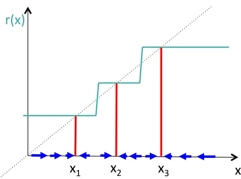
Regularized auto-encoders (see Bengio et al. 2012b for a review and a longer exposition) capture the structure of the training distribution thanks to the productive opposition be-tween reconstruction error and a regularizer. An auto-encoder maps inputsxto an internal representation (or code) f(x) through the encoder function f, and then maps back f(x) to the input space through a decoding function g. The composition of f and g is called the reconstruction function r, with r(x) = g(f(x)), and a reconstruction loss function ` penalizes the error made, with r(x) viewed as a prediction of x. When the auto-encoder is regularized, e.g., via a sparsity regularizer, a contractive regularizer (detailed below), or a denoising form of regularization (that we find below to be very similar to a contractive regularizer), the regularizer basically attempts to make r (orf) as simple as possible, i.e., as constant as possible, as unresponsive toxas possible. It means thatf has to throw away some information present in x, or at least represent it with less precision. On the other hand, to make reconstruction error small on the training set, examples that are neighbors on a high-density manifold must be represented with sufficiently different values off(x) or r(x). Otherwise, it would not be possible to distinguish and hence correctly reconstruct these examples. It means that the derivatives off(x) orr(x) in thex-directions along the manifold must remain large, while the derivatives (off orr) in thex-directions orthogonal to the manifold can be made very small. This is illustrated in Figure 1. In the case of prin-cipal components analysis, one constrains the derivative to be exactly 0 in the directions orthogonal to the chosen projection directions, and around 1 in the chosen projection di-rections. In regularized auto-encoders,f is non-linear, meaning that it is allowed to choose different principal directions (those that are well represented, i.e., ideally the manifold tan-gent directions) at differentx’s, and this allows a regularized auto-encoder with non-linear encoder to capture non-linear manifolds. Figure 2 illustrates the extreme case when the regularization is very strong (r wants to be nearly constant where density is high) in the special case where the distribution is highly concentrated at three points (three training ex-amples). It shows the compromise between obtaining the identity function at the training examples and having a flat r near the training examples, yielding a vector field r(x)−x that points towards the high density points.
x"
r(x)"
x
1"x
2"x
3"Figure 2: The reconstruction functionr(x) (in turquoise) which would be learned by a high-capacity auto-encoder on a 1-dimensional input, i.e., minimizing reconstruction errorat the train-ing examplesxi (withr(xi) in red) while trying to be as constant as possible otherwise.
The figure is used to exaggerate and illustrate the effect of the regularizer (corresponding to a largeσ2 in the loss function L later described by Equation 6. The dotted line is the identity reconstruction (which might be obtained without the regularizer). The blue arrows shows the vector field ofr(x)−xpointing towards high density peaks as estimated by the model, and estimating the score (log-density derivative), as shown in this paper.
rather than just the encoder, whose contraction penalty coefficient is the magnitude of the perturbation. This was first suggested in Rifai et al. (2011b).
The contractive auto-encoder, or CAE (Rifai et al., 2011b), is a particular form of reg-ularized auto-encoder which is trained to minimize the following regreg-ularized reconstruction error:
LCAE =E
"
`(x, r(x)) +λ
∂f(x) ∂x
2
F
#
(1)
where r(x) = g(f(x)) and ||A||2
F is the sum of the squares of the elements of A. Both the
squared loss`(x, r) =||x−r||2and the cross-entropy loss`(x, r) =−xlogr−(1−x) log(1−r) have been used, but here we focus our analysis on the squared loss because of the easier mathematical treatment it allows. Note that success in minimizing the CAE criterion strongly depends on the parameterization off andg and in particular on the tied weights constraint used, with f(x) = sigmoid(W x+b) andg(h) = sigmoid(WTh+c). The above regularizing term forcesf (as well as g, because of the tied weights) to be contractive, i.e., to have singular values less than 1.1 Larger values of λ yield more contraction (smaller singular values) where it hurts reconstruction error the least, i.e., in the local directions where there are only little or no variations in the data. These typically are the directions orthogonal to the manifold of high density concentration, as illustrated in Figure 2.
The denoising auto-encoder, or DAE (Vincent et al., 2008), is trained to minimize the following denoising criterion:
LDAE =E[`(x, r(N(x)))] (2)
where N(x) is a stochastic corruption of x and the expectation is over the training dis-tribution and the corruption noise source. Here we consider mostly the squared loss and Gaussian noise corruption, again because it is easier to handle them mathematically. In many cases, the exact same proofs can be applied to any kind of additive noise, but Gaussian noise serves as a good frame of reference.
Theorem 1 Letp be the probability density function of the data. If we train aDAE using the expected quadratic loss and corruption noise N(x) =x+with
∼ N 0, σ2I,
then the optimal reconstruction function r∗(x) will be given by
r∗(x) = E[p(x−)(x−)]
E[p(x−)] (3)
for values of x where p(x)6= 0.
Moreover, if we consider how the optimal reconstruction function r∗σ(x) behaves asymp-totically as σ →0, we get that
rσ∗(x) =x+σ2∂logp(x) ∂x +o(σ
2) as σ →0. (4)
The proof of this result is found in the Appendix. We make use of the small onotation throughout this paper and assume that the reader is familiar with asymptotic notation. In the context of Theorem 1, it has to be understood that all the other quantities except for σ are fixed when we study the effect of σ →0.
Equation 3 reveals that the optimal DAE reconstruction function at every point x is given by a kind of convolution involving the density function p, or weighted average from the points in the neighbourhood ofx, depending on how we would like to view it. A higher noise level σ means that a larger neighbourhood of x is taken into account. Note that the total quantity of “mass” being included in the weighted average of the numerator of (3) is found again at the denominator.
Gaussian noise is a simple case in the sense that it is additive and symmetrical, so it avoids the complications that would occur when trying to integrate over the density of pre-images x0 such that N(x0) = x for a given x. The ratio of those quantities that we have in Equation 3, however, depends strongly on the decision that we made to minimize the expected square error.
We get something even more interesting if we look at the second term of Equation 4 because it gives us an estimator of the score from
∂logp(x) ∂x = (r
∗
σ(x)−x)/σ2+o(1) as σ→0. (5)
This result is at the core of our paper. It is what allows us to start from a trained DAE, and then recover properties of the training density p(x) that can be used to sample from p(x).
Most of the asymptotic properties that we get by considering the limit as the Gaussian noise levelσ goes to 0 could be derived from a family of noise distribution that approaches a point mass distribution in a relatively “nice” way.
An interesting connection with contractive auto-encoders can also be observed by using a Taylor expansion of the denoising auto-encoder loss and assuming only thatrσ(x) =x+o(1)
asσ →0. In that case we get the following proposition.
Proposition 1 Letpbe the probability density function of the data. Consider aDAE using the expected quadratic loss and corruption noise N(x) =x+, with ∼ N 0, σ2I
. If we assume that the non-parametric solutions rσ(x) satisfies
rσ(x) =x+o(1) as σ →0,
then we can rewrite the loss as
LDAE =E
"
kr(x)−xk22+σ2
∂r(x) ∂x
2
F
#
+o(σ2) as σ→0.
The proof is in Appendix and uses a simple Taylor expansion aroundx.
Proposition 1 shows that the DAE with small corruption of variance σ2 is similar to a contractive auto-encoder with penalty coefficient λ = σ2 but where the contraction is imposed explicitly on the whole reconstruction function r(·) =g(f(·)) rather than on f(·) alone.2
This analysis motivates the definition of the reconstruction contractive auto-encoder (RCAE), a variation of the CAE where loss function is instead the squared reconstruction loss plus contractive penalty on the reconstruction:
LRCAE =E
"
kr(x)−xk2 2+σ2
∂r(x) ∂x
2
F
#
. (6)
This is an analytic version of the denoising criterion with small noise σ2, and also corre-sponds to a contractive auto-encoder with contraction on bothf andg, i.e., onr.
Because of the similarity between DAE and RCAE when taking λ = σ2 and because the semantics of σ2 is clearer (as a squared distance in input space), we will denote σ2 for the penalty term coefficient in situations involving RCAE. For example, in the statement of
Theorem 2, thisσ2 is just a positive constant; there is no notion of additive Gaussian noise, i.e., σ2 does not explicitly refer to a variance, but using the notationσ2 makes it easier to intuitively see the connection to the DAE setting.
The connection between DAE and RCAE established in Proposition 1 also serves as the basis for an alternative demonstration to Theorem 1 in which we study the asymptotic behavior of the RCAE solution. This result is contained in the following theorem.
Theorem 2 Let p be a probability density function that is continuously differentiable once and with support Rd (i.e., ∀x∈Rd we have p(x)6= 0). LetLσ2 be the loss function defined
by
Lσ2(r) =
Z
Rd
p(x) "
kr(x)−xk22+σ2
∂r(x) ∂x
2
F
#
dx (7)
for r :Rd → Rd assumed to be differentiable twice, and 0 ≤σ2 ∈ R used as factor to the
penalty term.
Let r∗σ2(x) denote the optimal function that minimizes Lσ2. Then we have that
rσ∗2(x) =x+σ2
∂logp(x) ∂x +o(σ
2) as σ2→0. (8)
Moreover, we also have the following expression for the derivative
∂rσ∗2(x)
∂x =I+σ
2∂2logp(x) ∂x2 +o(σ
2) as σ2 →0. (9)
Both these asymptotic expansions are to be understood in a context where we consider
r∗σ2(x) σ2≥0 to be a family of optimal functions minimizing Lσ2 for their corresponding
value of σ2. The asymptotic expansions are applicable point-wise in x, that is, with any fixed x we look at the behavior as σ2 →0.
The proof is given in the appendix and uses the Euler-Lagrange equations from the calculus of variations.
3. Minimizing the Loss to Recover Local Features of p(·)
One of the central ideas of this paper is that in a non-parametric setting (without parametric constraints onr), we have an asymptotic formula (as the noise levelσ →0) for the optimal reconstruction function for the DAE and RCAE that allows us to recover the score ∂log∂xp(x). A DAE is trained with a method that knows nothing about p, except through the use of training samples to minimize a loss function, so it comes as a surprise that we can compute the score of p at any pointx.
In the following subsections we explore the consequences and the practical aspect of this.
3.1 Empirical Loss
ˆ L= 1
N
N
X
n=1 r(x
(n))−x(n) 2 2+σ
2
∂r(x) ∂x
x=x(n)
2
F
!
based on a sample x(n) Nn=1 drawn from p(x).
Alternatively, the auto-encoder is trained online (by stochastic gradient updates) with a stream of examplesx(n), which corresponds to performing stochastic gradient descent on the expected loss (7). In both cases we obtain an auto-encoder that approximately minimizes the expected loss.
An interesting question is the following: what can we infer from the data-generating density when given an auto-encoder reconstruction functionr(x)?
The premise is that this auto-encoder r(x) was trained to approximately minimize a loss function that has exactly the form of (7) for some σ2 > 0. This is assumed to have been done through minimizing the empirical loss and the distribution p was only available indirectly through the samples x(n) Nn=1. We do not have access to p or to the samples. We have only r(x) and maybe σ2.
We will now discuss the usefulness of r(x) based on different conditions such as the model capacity and the value ofσ2.
3.2 Perfect World Scenario
As a starting point, we will assume that we are in a perfect situation, i.e., with no con-straint on r (non-parametric setting), an infinite amount of training data, and a perfect minimization. We will see what can be done to recover information about p in that ideal case. Afterwards, we will drop certain assumptions one by one and discuss the possible paths to getting back some information about p.
We use notationrσ2(x) when we want to emphasize the fact that the value ofr(x) came
from minimizing the loss with a certain fixed σ2.
Suppose thatrσ2(x) was trained with an infinite sample drawn fromp. Suppose also that
it had infinite (or sufficient) model capacity and that it is capable of achieving the minimum of the loss function (7) while satisfying the requirement that r(x) be twice differentiable. Suppose that we know the value ofσ2 and that we are working in a computing environment of arbitrary precision (i.e., no rounding errors).
As shown by Theorem 1 and Theorem 2, we would be able to get numerically the values of ∂log∂xp(x) at any point x∈Rd by simply evaluating
rσ2(x)−x
σ2 →
∂logp(x)
∂x as σ
2 →0. (10)
In the setup described, we do not get to pick values of σ2 so as to take the limit σ2 → 0. However, it is assumed thatσ2 is already sufficiently small that the above quantity is close to ∂log∂xp(x) for all intents and purposes.
3.3 Simple Numerical Example
both a DAE and an RCAE in this fashion by minimizing a discretized version of their losses defined by equations (2) and (6). The goal here is to show that, for either a DAE or RCAE, the approximation of the score that we get through Equation 5 gets arbitrarily close to the actual score ∂x∂ logp(x) as σ→0.
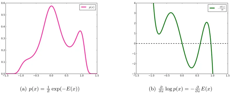
The distributionp(x) studied is shown in Figure 3 (left) and it was created to be simple enough to illustrate the mechanics. We plotp(x) in Figure 3 (left) along with the score of p(x) (right).
(a)p(x) = 1
Zexp(−E(x)) (b) ∂
∂xlogp(x) =− ∂ ∂xE(x)
Figure 3: The density p(x) and its score for a simple one-dimensional example.
The model ˆr(x) is fitted by dividing the interval [−1.5,1.5] into M = 1000 partition pointsx1, . . . , xM evenly separated by a distance ∆. The discretized version of the RCAE
loss function is
M
X
i=1
p(xi)∆ (ˆr(xi)−xi)2+σ2 M−1
X
i=1
p(xi)∆
ˆ
r(xi+1)−r(xˆ i)
∆
2
. (11)
Every value ˆr(xi) fori= 1, . . . , M is treated as a free parameter. Setting to 0 the derivative
with respect to the ˆr(xi) yields a system of linear equations in M unknowns that we can
solve exactly. From that RCAE solution ˆr we get an approximation of the score ofpat each point xi. A similar thing can be done for the DAE by using a discrete version of the exact
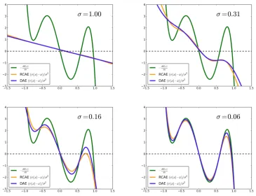
solution (3) from Theorem 1. We now have two ways of approximating the score ofp. In Figure 4 we compare the approximations to the actual score of p for decreasingly small values ofσ ∈ {1.00,0.31,0.16,0.06}.
3.4 Vector Field Around a Manifold
Figure 4: Comparing the approximation of the score of p given by discrete versions of optimally trained auto-encoders with infinite capacity. The approximations given by the RCAE are in orange while the approximations given by the DAE are in purple. The results are shown for decreasing values ofσ∈ {1.00,0.31,0.16,0.06} that have been selected for their visual appeal.
As expected, we see in that the RCAE (orange) and DAE (purple) approximations of the score are close to each other as predicted by Proposition 1. Moreover, they are also converging to the true score (green) as predicted by Theorem 1 and Theorem 2.
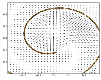
Two-dimensional data points (x, y) were generated along a spiral according to the fol-lowing equations:
x= 0.04 sin(t), y= 0.04 cos(t), t∼Uniform (3,12).
The non-convexity of the problem makes it such that the solution found depends on the initialization parameters. The random corruption noise used can also influence the final outcome. Moreover, the fact that we are using a finite training sample size with reasonably small noise may allow for undesirable behavior of r in regions far away from the training samples. For those reasons, we trained the model multiple times and selected two of the most visually appealing outcomes. These are found in Figure 5 which features a more global perspective along with a close-up view.
(a)r(x)−xvector field, acting as sink, zoomed out (b) r(x)−xvector field, close-up
Figure 5: The original 2-D data from the data-generating density p(x) is plotted along with the vector field defined by the values ofr(x)−x for trained auto-encoders (corresponding to the estimation of the score ∂log∂xp(x)).
sign: on one side of the median they point to one of the high-density regions while on the other side they point to the other, as clearly visible in Figure 5(b) between the arms of the spiral.
We believe that this analysis is valid not just for contractive and denoising auto-encoders, but for regularized auto-encoders in general. The intuition behind this statement can be firmed up by analyzing Figure 2: the score-like behavior ofr(x)−xarises simply out of the opposing forces of (a) trying to make r(x) =x at the training examples and (b) trying to make r(x) as regularized as possible (as close to a constant as possible).
Note that previous work (Rifai et al., 2012; Bengio et al., 2013b) has already shown that contractive auto-encoders (especially when they are stacked in a way similar to RBMs in a deep belief net) learn good models of high-dimensional data (such as images), and that these models can be used not just to obtain good representations for classification tasks but that good quality samples can be obtained from the model, by a random walk near the manifold of high-density. This was achieved by essentially following the vector field and adding noise along the way.
3.5 Missing σ2
When we are in the same setting as in Section 3.2 but the value ofσ2 is unknown, we can modify (10) a bit and avoid dividing by σ2. That is, for a trained reconstruction function r(x) given to us we just take the quantityr(x)−xand it should be approximately the score up to a multiplicative constant. We get that
r(x)−x∝ ∂logp(x) ∂x .
Equivalently, if one estimates the density via an energy function (minus the unnormalized log density), thenx−r(x) estimates the derivative of the energy function.
We still have to assume that σ2 is small. Otherwise, if the unknownσ2 is too large we might get a poor estimation of the score.
3.6 Limited Parameterization
We should also be concerned about the fact that r(x)−x is trying to approximate−∂E∂x(x) asσ2 →0 but we have not made any assumptions about the space of functions that r can represent when we are dealing with a specific implementation.
When using a certain parameterization of r such as the one from Section 3.3, there is no guarantee that the family of functions in which we selectr each represent a conservative vector field (i.e., the gradient of a potential function). Even if we start from a density p(x) ∝exp(−E(x)) and we have thatr(x)−x is very close to −∂x∂ E(x) in terms of some given norm, there is not guarantee that there exists an associated function E0(x) for which r(x)−x∝ −∂
∂xE0(x) andE0(x)≈E(x).
Conceptually, another way to see this is to argue that if such a function E0(x) existed, its second-order mixed derivatives should be equal. That is, we should have that
∂2E0(x) ∂xi∂xj
= ∂ 2E0(x) ∂xj∂xi
∀i, j,
which is equivalent to
∂ri(x)
∂xj
= ∂rj(x) ∂xi
∀i, j.
Again in the context of Section 3.3, with the parameterization used for that particular kind of denoising auto-encoder, this would yield the constraint that VT = W. That is, unless we are using tied weights, we know that no such potentialE0(x) exists, and yet when running the experiments from Section 3.3 we obtained much better results with untied weights. To make things worse, it can also be demonstrated that the energy function that we get from tied weights leads to a distribution that is not normalizable (it has a divergent integral over Rd). In that sense, this suggests that we should not worry too much about
the exact parameterization of the denoising auto-encoder as long as it has the required flexibility to approximate the optimal reconstruction function sufficiently well.
3.7 Relation to Denoising Score Matching
There is a connection between our results and previous research involving score matching for denoising auto-encoders. We will summarize here the existing results from Vincent (2011) and show that, whereas they have shown that denoising auto-encoders with a particular form estimated the score, our results extend this to a very large family of estimators (including the non-parametric case). This will provide some reassurance given some of the potential issues mentioned in Section 3.6.
Motivated by the analysis of denoising auto-encoders, the authors of Vincent (2011) are concerned with the case where we explicitly parameterize an energy functionE(x), yielding an associated score function ψ(x) = −∂E(∂xx) and we stochastically corrupt the original samplesx ∼p to obtain noisy samples ˜x ∼qσ(˜x|x). In particular, the article analyzes the
case where qσ adds Gaussian noise of varianceσ2 tox. The main result is that minimizing
the expected square difference betweenψ(˜x) and the score of qσ(˜x|x),
Ex,x˜ "
ψ(˜x)−∂logqσ(˜x|x) ∂˜x
2# ,
is equivalent to performingscore matching(Hyv¨arinen, 2005) with estimatorψ(˜x) and target density qσ(˜x) =
R
qσ(˜x|x)p(x)dx, where p(x) generates the training samples x. Note that
when a finite training set is used, qσ(˜x) is simply a smooth of the empirical distribution
(e.g., the Parzen density with Gaussian kernel of width σ). When the corruption noise is Gaussian, qσ(˜x|x)
∂x˜ =
x−˜x
σ2 , from which we can deduce that if we define a reconstruction
function
r(˜x) = ˜x+σ2ψ(˜x), (12) then the above expectation is equivalent to
Ex,x˜ "
r(˜x)−x˜ σ2 −
x−x˜ σ2
2# = 1
σ2Ex,˜x h
which is the denoising criterion. This says that when the reconstruction function r is pa-rameterized so as to correspond to the scoreψof a model density (as per Equation 12, and whereψis a derivative of some log-density), the denoising criterion onr with Gaussian cor-ruption noise is equivalent to score matching with respect to a smooth of the data-generating density, i.e., a regularized form of score matching. Note that this regularization appears desirable, because matching the score of the empirical distribution (or an insufficiently smoothed version of it) could yield undesirable results when the training set is finite. Since score matching has been shown to be a consistent induction principle (Hyv¨arinen, 2005), it means that thisdenoising score matching(Vincent, 2011; Kingma and LeCun, 2010; Swer-sky et al., 2011) criterion recovers the underlying density, up to the smoothing induced by the noise of variance σ2. By making σ2 small, we can make the estimator arbitrarily good (and we would expect to want to do that as the amount of training data increases). Note the correspondence of this conclusion with the results presented here, which show (1) the equivalence between the RCAE’s regularization coefficient and the DAE’s noise varianceσ2, and (2) that minimizing the equivalent analytic criterion (based on a contraction penalty) estimates the score when σ2 is small. The difference is that our result holds even when r is not parameterized as per Equation 12, i.e., is not forced to correspond with the score function of a density.
3.8 Estimating the Hessian
Since we have r(xσ)−2 x as an estimator of the score, we readily obtain that the Hessian of
the log-density, can be estimated by the Jacobian of the reconstruction function minus the identity matrix:
∂2logp(x) ∂x2 ≈(
∂r(x)
∂x −I)/σ 2 as shown by Equation 9 of Theorem 2.
In spite of its simplicity, this result is interesting because it relates the derivative of the reconstruction function, i.e., a Jacobian matrix, with the second derivative of the log-density (or of the energy). This provides insights into the geometric interpretation of the reconstruction function when the density is concentrated near a manifold. In that case, near the manifold the score is nearly 0 because we are near a ridge of density, and the density’s second derivative matrix tells us in which directions the first density remains close to zero or increases. The ridge directions correspond to staying on the manifold and along these directions we expect the second derivative to be close to 0. In the orthogonal directions, the log-density should decrease sharply while its first and second derivatives would be large in magnitude and negative in directions away from the manifold.
Returning to the above equation, keep in mind that in these derivations σ2 is near 0 and r(x) is near x, so that ∂r∂x(x) is close to the identity. In particular, in the ridge (manifold) directions, we should expect ∂r∂x(x) to be closer to the identity, which means that the reconstruction remains faithful (r(x) =x) when we move on the manifold, and this corresponds to the eigenvalues of ∂r∂x(x)that are near 1, making the corresponding eigenvalues of ∂2log∂x2p(x) near 0. On the other hand, in the directions orthogonal to the manifold,
∂r(x)
∂x
Besides first and second derivatives of the density, other local properties of the density are its local mean and local covariance, discussed in the Appendix, Section D.
4. Sampling with Metropolis-Hastings
In this section we show how a technique to generate samples from a given denoising auto-encoder by using Metropolis-Hastings.
We start by explaining how to compute differences in energies Section 4.1, and then we use this in Section 4.2 to generate samples. We provide an experimental example and we discuss the potential problems that this method has.
This section serves as a demonstration that the main result of this paper, i.e., the connection between denoising auto-encoders and the score ∂log∂xp(x), is more than just an observation : it can have practical uses.
4.1 Estimating Energy Differences
One of the immediate consequences of Theorem 2 and Equation 10 is that, while we cannot easily recover the energy E(x) itself, it is possible to approximate the energy difference E(x∗)−E(x) between two statesx and x∗. This can be done by using a first-order Taylor approximation
E(x∗)−E(x) = ∂E(x) ∂x
T
(x∗−x) +o(kx∗−xk).
To get a more accurate approximation, we can also use a path integral fromxtox∗ that we can discretize in sufficiently many steps. With a smooth path γ(t) : [0,1]→ Rd, assuming
thatγ stays in a region where our DAE/RCAE can be used to approximate ∂E∂x well enough, we have that
E(x∗)−E(x) = Z 1
0
∂E ∂x (γ(t))
T
γ0(t)dt. (13)
The simplest way to discretize this path integral is to pick points {xi}ni=1 spread at even distances on a straight line from x1 =x toxn=x∗. We approximate (13) by
E(x∗)−E(x)≈ 1 n
n
X
i=1
∂E ∂x (xi)
T
(x∗−x) (14)
4.2 Sampling
With Equation 13 from Section 4.1 we can perform approximate sampling from the es-timated distribution, using the score estimator to approximate energy differences which are needed in the Metropolis-Hastings accept/reject decision. Using a symmetric proposal q(x∗|x), the acceptance ratio is
α= p(x ∗)
p(x) = exp(−E(x
∗) +E(x))
estimator of ∂E∂x. An example of this process is shown in Figure 6 in which we sample from a density concentrated around a 1-d manifold embedded in a space of dimension 10. For this particular task, we have trained only DAEs and we are leaving RCAEs out of this exercise. Given that the data is roughly contained in the range [−1.5,1.5] along all dimensions, we selected a training noise level σtrain = 0.1 so that the noise would have an appreciable effect while still being relatively small. As required by Theorem 1, we have used isotropic Gaussian noise of varianceσtrain2 .
The Metropolis-Hastings proposal q(x∗|x) = N(0, σMH2 I) has a noise parameter σMH that needs to be set. In the situation shown in Figure 6, we used σMH = 0.1. After some hyperparameter tweaking and exploring various scales forσtrain, σMH, we found that setting both to be 0.1 worked well.
When σtrain is too large, the DAE trained learns a “blurry” version of the density that fails to represent the details that we are interested in. The samples shown in Figure 6 are very convincing in terms of being drawn from a distribution that models well the original density. We have to keep in mind that Theorem 2 describes the behavior as σtrain →0 so we would expect that the estimator becomes worse when σtrain is taking on larger values. In this particular case with σtrain = 0.1, it seems that we are instead modeling something like the original density to which isotropic Gaussian noise of varianceσtrain2 has been added. In the other extreme, when σtrain is too small, the DAE is not exposed to any training example farther away from the density manifold. This can lead to various kinds of strange behaviors when the sampling algorithm falls into those regions and then has no idea what to do there and how to get back to the high-density regions. We come back to that topic in Section 4.3.
It would certainly be possible to pick both a very small value for σtrain =σMH = 0.01 to avoid the spurious maxima problem illustrated in Section 4.3. However, this leads to the same kind of mixing problems that any kind of MCMC algorithm has. Smaller values of σMH lead to higher acceptance ratios but worse mixing properties.
4.3 Spurious Maxima
There are two very real concerns with the sampling method discussed in Section 4.2. The first problem is with the mixing properties of MCMC and it is discussed in that section. The second issue is with spurious probability maxima resulting from inadequate training of the DAE. It happens when an auto-encoder lacks the capacity to model the density with enough precision, or when the training procedure ends up in a bad local minimum (in terms of the DAE parameters).
This is illustrated in Figure 7 where we show an example of a vector field r(x)−x for a DAE that failed to properly learn the desired behavior in regions away from the spiral-shaped density.
5. Conclusion
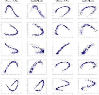
con-original sampled original sampled
Figure 6: Samples drawn from the estimate of ∂E∂x given by a DAE by the Metropolis-Hastings method presented in Section 4. By design, the data density distribu-tion is concentrated along a 1-d manifold embedded in a space of dimension 10. This data can be visualized in the plots above by plotting pairs of dimensions (x0, x1), . . . ,(x8, x9),(x9, x0), going in reading order from left to right and then line by line. For each pair of dimensions, we show side by side the original data (left) with the samples drawn (right).
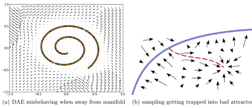
(a) DAE misbehaving when away from manifold (b) sampling getting trapped into bad attractor
Figure 7: (a) On the left we show a r(x)−x vector field similar to that of the earlier Figure 5. The density is concentrated along a spiral manifold and we should have the reconstruction functionr bringing us back towards the density. In this case, it works well in the region close to the spiral (the magnitude of the vectors is so small that the arrows are shown as dots). However, things are out of control in the regions outside. This is because the level of noise used during training was so small that not enough of the training examples were found in those regions. (b) On the right we sketch what may happen when we follow a sampling procedure as described in Section 4.2. We start in a region of high density (in purple) and we illustrate in red the trajectory that our samples may take. In that situation, the DAE/RCAE was not trained properly. The resulting vector field does not reflect the density accurately because it should not have this attractor (i.e., stable fixed point) outside of the manifold on which the density is concentrated. Conceptually, the sampling procedure visits that spurious attractor because it assumes that it corresponds to a region of high probability. In some cases, this effect is regrettable but not catastrophic, but in other situations we may end up with completely unusable samples. In the experiments, training with enough of the examples involving sufficiently large corruption noise typically eliminates that problem.
Vincent, 2011). Toy experiments have confirmed that a good estimator of the density can be obtained when this criterion is non-parametrically minimized. The experiments have also confirmed that an MCMC could be setup that approximately samples from the estimated model, by estimating energy differences to first order (which only requires the score) to perform approximate Metropolis-Hastings MCMC.
More generally, we would like to generalize to any form of reconstruction error (for exam-ple many imexam-plementations of auto-encoders use a Bernoulli cross-entropy as reconstruction loss function) and any (reasonable) form of corruption noise (many implementations use masking or salt-and-pepper noise, not just Gaussian noise). More fundamentally, the need to rely onσ→0 is troubling, and getting rid of this limitation would also be very useful. A possible solution to this limitation, as well as adding the ability to handle both discrete and continuous variables, has recently been proposed while this article was under review (Bengio et al., 2013a).
It would also be interesting to generalize the results presented here to other regularized auto-encoders besides the denoising and contractive types. In particular, the commonly used sparse auto-encoders seem to fit the qualitative pattern illustrated in 2 where a score-like vector field arises out of the opposing forces of minimizing reconstruction error and regularizing the auto-encoder.
We have mostly considered the harder case where the auto-encoder parameterization does not guarantee the existence of an analytic formulation of an energy function. It would be interesting to compare experimentally and study mathematically these two formulations to assess how much is lost (because the score function may be somehow inconsistent) or gained (because of the less constrained parameterization).
Acknowledgments
The authors thank Salah Rifai Max Welling, Yutian Chen and Pascal Vincent for fruitful discussions, and acknowledge the funding support from NSERC, Canada Research Chairs and CIFAR.
Appendix A. Exact Solution for DAE
There is a way to get an exact solution to the DAE loss (2) without assuming that σ →0 or that the noise is Gaussian (but still using the quadratic loss).
We let p be the density function of the data such that ∀x ∈ Rd, p(x) > 0, and we use
additive isotropic Gaussian noise of variance σ2. We are in the non-parametric setting in which we are minimizing
LDAE= Z
Rd
E∼N(0,σ2I)
h
p(x)kr(x+)−xk22idx (15) with respect to the function r:Rd→Rd.
By using an auxiliary variable ˜x = x+, we can rewrite this loss in a way that puts the quantity r(˜x) in focus and allows us to perform the minimization with respect to each choice ofr(˜x) independently. That is, we have that
LDAE= Z
Rd
E∼N(0,σ2I)
h
0 =E∼N(0,σ2I)[p(˜x−)r∗(˜x)−x˜+] (17)
E∼N(0,σ2I)[p(˜x−)r∗(˜x)] =E∼N(0,σ2I)[p(˜x−)(˜x−)] (18)
r∗(˜x) = E∼N(0,σ2I)[p(˜x−)(˜x−)]
E∼N(0,σ2I)[p(˜x−)]
(19)
Conceptually, this means that the optimal DAE reconstruction function at every point ˜
x∈Rdis given by a kind of convolution involving the density functionp, or weighted average
from the points in the neighbourhood of ˜x, depending on how we would like to view it. A higher noise level σ means that a larger neighbourhood of ˜x is taken into account. Note that the total quantity of “mass” being included in the weighted average of the numerator of (19) is found again at the denominator.
Appendix B. Relationship between Contractive Penalty and Denoising Criterion
Theorem 1 When using corruption noiseN(x) =x+with
∼ N 0, σ2I, the objective function LDAE is
LDAE= Ekx−r(x)k2+σ2E
"
∂r(x) ∂x
2
F
#!
+o(σ2) as σ→0.
Proof With a Taylor expansion around x we have that
r(x+) =r(x) +∂r(x)
∂x +o(σ 2). Substituting this into LDAE we have that
LDAE =E
1 2
x−
r(x) +∂r∂x(x)+o(σ2)
2
=
Ekx−r(x)k2−2E[]TE
∂r(x)
∂x T
(x−r(x))
+T r
ETE
∂r(x)
∂x
T ∂r(x)
∂x
+o(σ2) = 12
Ekx−r(x)k2+σ2E
∂r(x)
∂x
2
F
+o(σ2) (20)
Appendix C. Calculus of Variations
Theorem 2 Let p be a probability density function that is continuously differentiable once and with support Rd (i.e., ∀x∈Rd we have p(x)6= 0). LetLσ2 be the loss function defined
by
Lσ2(r) =
Z
Rd
p(x) "
kr(x)−xk22+σ2 ∂r(x) ∂x 2 F # dx
for r :Rd → Rd assumed to be differentiable twice, and 0 ≤σ2 ∈ R used as factor to the
penalty term.
Let r∗σ2(x) denote the optimal function that minimizes Lσ2. Then we have that
rσ∗2(x) =x+σ2
∂logp(x) ∂x +o(σ
2) as σ2→0. Moreover, we also have the following expression for the derivative
∂rσ∗2(x)
∂x =I+σ
2∂2logp(x) ∂x2 +o(σ
2) as σ2 →0.
Both these asymptotic expansions are to be understood in a context where we consider
r∗σ2(x) σ2≥0 to be a family of optimal functions minimizing Lσ2 for their corresponding
value of σ2. The asymptotic expansions are applicable point-wise in x, that is, with any fixed x we look at the behavior as σ2 →0.
Proof
This proof is done in two parts. In the first part, the objective is to get to Equation 23 that has to be satisfied for the optimum solution.
We will leave out theσ2indices from the expressions involvingr(x) to make the notation lighter. We have a more important need for indiceskinrk(x) that denote thedcomponents
of r(x)∈Rd.
We treat σ2 as given and constant for the first part of this proof.
In the second part we work out the asymptotic expansion in terms ofσ2. We again work with the implicit dependence of r(x) on σ2.
(part 1 of the proof )
We make use of the Euler-Lagrange equation from the Calculus of Variations. We would refer the reader to either (Dacorogna, 2004) or Wikipedia for more on the topic. Let
f(x1, . . . , xn, r, rx1, . . . , rxn) =p(x) "
kr(x)−xk22+σ2 ∂r(x) ∂x 2 F #
wherex= (x1, . . . , xd) , r(x) = (r1(x), . . . , rd(x)) andrxi =
∂f ∂xi. We can rewrite the lossL(r) more explicitly as
L(r) = Z Rd p(x) d X i=1
(ri(x)−xi)2+σ2 d X i=1 d X j=1 ∂ri(x)
∂xj 2 dx = d X i=1 Z Rd p(x)
(ri(x)−xi)2+σ2 d
X
j=1 ∂ri(x)
∂xj
2
to observe that the componentsr1(x), . . . , rd(x) can each be optimized separately.
The Euler-Lagrange equation to be satisfied at the optimal r :Rd→Rd is
∂f ∂r = d X i=1 ∂ ∂xi ∂f ∂rxi
.
In our situation, the expressions from that equation are given by
∂f
∂r = 2(r(x)−x)p(x)
∂f ∂rxi
= 2σ2p(x) h
∂r1
∂xi
∂r2
∂xi · · ·
∂rd ∂xi iT ∂ ∂xi ∂f ∂rxi
= 2σ2∂p(x) ∂xi
h
∂r1
∂xi
∂r2
∂xi · · ·
∂rd
∂xi iT
+2σ2p(x)h ∂2r1
∂x2
i
∂2r 2
∂x2
i
· · · ∂2rd
∂x2
i iT
and the equality to be satisfied at the optimum becomes
(r(x)−x)p(x) =σ2
d X i=1
∂p(x)
∂xi
∂r1
∂xi +p(x)
∂2r1
∂x2
i ..
.
∂p(x)
∂xi
∂rd
∂xi +p(x)
∂2r
d ∂x2 i . (22)
As Equation 21 hinted, the expression (22) can be decomposed into the different com-ponentsrk(x) :Rd→R that maker. Fork= 1, . . . , dwe get
(rk(x)−xk)p(x) =σ2 d X i=1 ∂p(x) ∂xi
∂rk(x)
∂xi
+p(x)∂ 2r k(x) ∂x2 i .
Asp(x)6= 0 by hypothesis, we can divide all the terms byp(x) and note that∂p∂x(x)
i /p(x) =
∂logp(x)
∂xi .
We get
rk(x)−xk=σ2 d
X
i=1
∂logp(x) ∂xi
∂rk(x)
∂xi
+∂ 2r
k(x)
∂x2i
. (23)
This first thing to observe is that when σ2 = 0 the solution is just rk(x) = xk, which
translates intor(x) =x. This is not a surprise because it represents the perfect reconstruc-tion value that we get when we the penalty term vanishes in the loss funcreconstruc-tion.
This linear partial differential Equation 23 can be used as a recursive relation for rk(x)
to obtain a Taylor series in σ2. The goal is to obtain an expression of the form
r(x) =x+σ2h(x) +o(σ2) as σ2 →0 (24) where we can solve for h(x) and for which we also have that
∂r(x)
∂x =I+σ 2∂h(x)
∂x +o(σ
2) as σ2 →0.
We can substitute in the right-hand side of Equation 24 the value for rk(x) that we get
from Equation 24 itself. This substitution would be pointless in any other situation where we are not trying to get a power series in terms ofσ2 around 0.
rk(x) =xk +σ2 d
X
i=1
∂logp(x) ∂xi
∂rk(x)
∂xi +∂ 2r k(x) ∂x2 i
=xk +σ2 d
X
i=1
∂logp(x) ∂xi
∂ ∂xi
xk+σ2 d
X
j=1
∂logp(x) ∂xj
∂rk(x)
∂xj +∂ 2r k(x) ∂x2 j ! +σ2 d X i=1 ∂2r
k(x)
∂x2i =xk +σ2
d
X
i=1
∂logp(x) ∂xi I
(i=k) +σ2
d
X
i=1
∂2rk(x)
∂x2i +σ22 d X i=1 d X j=1
∂logp(x) ∂xi
∂ ∂xi
∂logp(x) ∂xj
∂rk(x)
∂xj +∂ 2r k(x) ∂x2 j !!
rk(x) =xk +σ2
∂logp(x) ∂xk
+σ2
d
X
i=1
∂2rk(x)
∂x2
i
+σ22ρ(σ2, x)
Now we would like to get rid of that σ2Pd
i=1
∂2rk(x)
∂x2
i term by showing that it is a term that involves only powers of σ22 or higher. We get this by showing what we get by differentiating the expression for rk(x) in line (25) twice with respect to somel.
∂rk(x)
∂xl
=I(i=l) +σ2∂
2logp(x) ∂xl∂xk
+σ2 ∂ ∂xl
d
X
i=1
∂2rk(x)
∂x2
i
+σ2ρ(σ2, x) !
∂2rk(x)
∂x2l =σ
2∂3logp(x) ∂x2l∂xk
+σ2 ∂ ∂x2l
d
X
i=1
∂2rk(x)
∂x2i +σ
2ρ(σ2, x) !
Since σ2 is a common factor in all the terms of the expression of ∂2rk(x)
∂x2
l
we get what we needed. That is,
rk(x) =xk+σ2
∂logp(x) ∂xk
This shows that
r(x) =x+σ2∂logp(x) ∂x +o(σ
2) as σ2 →0 and
∂r(x)
∂x =I+σ
2∂2logp(x) ∂x2 +o(σ
2) as σ2 →0 which completes the proof.
Appendix D. Local Mean
In preliminary work (Bengio et al., 2012a), we studied how the optimal reconstruction could possibly estimate so-called local moments. We revisit this question here, with more appealing and precise results.
What previous work on denoising and contractive auto-encoders suggest is that regu-larized auto-encoders cancapture the local structure of the densitythrough the value of the encoding (or reconstruction) function and its derivative. In particular, Rifai et al. (2012); Bengio et al. (2012a) argue that the first and second derivatives tell us in which directions it makes sense to randomly move while preserving or increasing the density, which may be used to justify sampling procedures. This motivates us here to study so-called local moments as captured by the auto-encoder, and in particular the local mean, following the definitions introduced in Bengio et al. (2012a).
D.1 Definitions for Local Distributions
Let p be a continuous probability density function with support Rd. That is, ∀x ∈ Rd
we have that p(x) 6= 0. We define below the notion of a local ball Bδ(x0), along with an associatedlocal density, which is the normalized product ofpwith the indicator for the ball:
Bδ(x0) = {x s.t. kx−x0k2 < δ} Zδ(x0) =
Z
Bδ(x0)
p(x)dx
pδ(x|x0) = 1 Zδ(x0)
p(x)I(x∈Bδ(x0))
where Zδ(x0) is the normalizing constant required to make pδ(x|x0) a valid pdf for a
distribution centered on x0. The support of pδ(x|x0) is the ball of radius δ around x0 denoted by Bδ(x0). We stick to the 2-norm in terms of defining the ballsBδ(x0) used, but everything could be rewritten in terms of anotherp-norm to have slightly different formulas. We use the following notation for what will be referred to as the first twolocal moments (i.e., local mean and local covariance) of the random variable described by pδ(x|x0).
mδ(x0) def
= Z
Rd
xpδ(x|x0)dx
Cδ(x0) def
= Z
Rd
(x−mδ(x0))(x−mδ(x0))Tpδ(x|x0)dx
Theorem 3 Let pbe of class C3 and represent a probability density function. Letx0∈Rd
with p(x0)6= 0. Then we have that
mδ(x0) =x0+δ2 1 d+ 2
∂logp(x) ∂x x0
+o δ3 .
This links the local mean of a density with the score associated with that density. Combining this theorem with Theorem 2, we obtain that the optimal reconstruction function r∗(·) also estimates the local mean:
mδ(x)−x=
δ2 σ2(d+ 2)(r
∗(x)−x) +A(δ) +δ2B(σ2) (25)
for error terms A(δ), B(σ2) such that
A(δ)∈o(δ3) as δ→0, B(σ2)∈o(1) as σ2→0.
This means that we can loosely estimate thedirectionto the local mean by the direction of the reconstruction:
mδ(x)−x ∝ r∗(x)−x. (26)
Appendix E. Asymptotic formulas for localized moments
Proposition 4 Let p be of classC2 and let x0 ∈Rd. Then we have that
Zδ(x0) =δd
πd/2 Γ (1 +d/2)
p(x0) +δ2Tr(H(x0)) 2(d+ 2) +o(δ
3)
where H(x0) = ∂2∂xp(2x)
x=x0
. Moreover, we have that
1 Zδ(x0)
=δ−dΓ (1 +d/2) πd/2
1 p(x0)
−δ2 1 p(x0)2
Tr(H(x0)) 2(d+ 2) +o(δ
3)
.
Proof
Zδ(x0) =
Z
Bδ(x0)
"
p(x0) + ∂p(x) ∂x x0
(x−x0) + 1
2!(x−x0)
TH(x0)(x−x0)
+1 3!D
(3)p(x0)(x−x0) +o(δ3)
dx
= p(x0) Z
Bδ(x0)
dx + 0 + 1 2
Z
Bδ(x0)
(x−x0)TH(x0)(x−x0)dx + 0 + o(δd+3)
= p(x0)δd
πd/2
Γ (1 +d/2)+δ
d+2 πd/2
4Γ (2 +d/2)Tr (H(x0)) +o(δ
d+3)
= δd π
d/2 Γ (1 +d/2)
p(x0) +δ2Tr(H(x0)) 2(d+ 2) +o(δ
We use Proposition 10 to get that trace come up from the integral involvingH(x0). The expression for 1/Zδ(x0) comes from the fact that, for anya, b >0 we have that
1
a+bδ2+o(δ3) =
a−1
1 +abδ2+o(δ3) = 1 a
1−(b
aδ
2+o(δ3)) +o(δ4)
= 1 a−
b a2δ
2+o(δ3) asδ→0.
by using the classic result from geometric series where 1+1r = 1−r+r2−. . .for|r|<1. Now we just apply this to
1 Zδ(x0)
=δ−dΓ (1 +d/2) πd/2
1 h
p(x0) +δ2 Tr(2(Hd+2)(x0)) +o(δ3) i
and get the expected result.
Theorem 5 Let pbe of class C3 and represent a probability density function. Letx0∈Rd
with p(x0)6= 0. Then we have that
mδ(x0) =x0+δ2
1 d+ 2
∂logp(x) ∂x x0
+o δ3.
Proof
The leading term in the expression for mδ(x0) is obtained by transforming the xin the integral into ax−x0 to make the integral easier to integrate.
mδ(x0) =
1 Zδ(x0)
Z
Bδ(x0)
xp(x)dx=x0+ 1 zδ(x0)
Z
Bδ(x0)
(x−x0)p(x)dx.
Now using the Taylor expansion around x0
mδ(x0) = x0+ 1 Zδ(x0)
Z
Bδ(x0)
(x−x0) "
p(x0) + ∂p(x) ∂x x0
(x−x0)
+1
2(x−x0)
T ∂2p(x)
∂x2 x0
(x−x0) +o(kx−x0k2) #
dx.
Remember that R
Bδ(x0)f(x)dx= 0 whenever we have a function f is anti-symmetrical
(or “odd”) relative to the pointx0(i.e.,f(x−x0) =f(−x−x0)). This applies to the terms (x−x0)p(x0) and (x−x0)(x−x0) ∂
2p(x)
∂x2
x=x0
mδ(x0) = x0+
1 Zδ(x0)
Z
Bδ(x0)
"
(x−x0)T ∂p(x) ∂x x0
(x−x0) +o(kx−x0k3) #
dx
= x0+ 1 Zδ(x0)
δd+2 π d
2
2Γ 2 + d2 ! ∂p(x) ∂x x0
+o(δ3).
Now, looking at the coefficient in front of ∂p∂x(x)
x0
in the first term, we can use
Propo-sition 4 to rewrite it as
1 Zδ(x0)
δd+2 π d
2
2Γ 2 +d2 !
= δ−dΓ (1 +d/2) πd/2
1 p(x0)
−δ2 1 p(x0)2
Tr(H(x0)) 2(d+ 2) +o(δ
3)
δd+2 π d
2
2Γ 2 + d2 = δ2 Γ 1 +
d
2
2Γ 2 + d2
1 p(x0) −δ
2 1 p(x0)2
Tr(H(x0)) 2(d+ 2) +o(δ
3)
=δ2 1 p(x0)
1
d+ 2+o(δ 3).
There is no reason the keep the −δ4 Γ(1+ d
2)
2Γ(2+d2) 1
p(x0)2
Tr(H(x0))
2(d+2) in the above expression be-cause the asymptotic error from the remainder term in the main expression is o(δ3). That would swallow our exact expression forδ4 and make it useless.
We end up with
mδ(x0) =x0+δ2 1 d+ 2
∂logp(x) ∂x x0
+o(δ3).
Appendix F. Integration on balls and spheres
This result comes fromMulti-dimensional Integration : Scary Calculus Problems from Tim Reluga (who got the results from How to integrate a polynomial over a sphere by Gerald B. Folland).
Theorem 6 Let B = n
x∈Rd
Pd
j=1x2j ≤1
o
be the ball of radius 1 around the origin. Then Z B d Y j=1
|xj|ajdx=
Q Γ a j+1 2
Γ 1 + d2+ 12P aj
Corollary 7 Let B be the ball of radius1 around the origin. Then
Z
B d
Y
j=1 xaj
j dx=
Q Γ
aj+1
2
Γ(1+d2+12P
aj) if all the aj are even integers
0 otherwise
for any non-negative integers aj ≥0. Note the absence of the absolute values put on the
xaj
j terms.
Corollary 8 Let Bδ(0)⊂Rd be the ball of radius δ around the origin. Then
Z
Bδ(0)
d
Y
j=1
xajjdx=
δd+Paj
Q
Γaj2+1 Γ(1+d
2+ 1 2
P
aj) if all theajare even integers
0 otherwise
for any non-negative integers aj ≥0. Note the absence of the absolute values on thex aj
j
terms.
Proof
We take the theorem as given and concentrate here on justifying the two corollaries. Note how in Corollary 7 we dropped the absolute values that were in the original Theo-rem 6. In situations where at least oneaj is odd, we have that the functionf(x) =Qdj=1x
aj
j
becomes odd in the sense that f(−x) = −f(x). Because of the symmetrical nature of the integration on the unit ball, we get that the integral is 0 as a result of cancellations.
For Corollary 8, we can rewrite the integral by changing the domain with yj =xj/δ so
that
δ−Paj Z
Bδ(0)
d
Y
j=1
xajjdx= Z
Bδ(0)
d
Y
j=1
(xj/δ)ajdx=
Z
B1(0)
d
Y
j=1
yajδddy.
We pull out the δd that we got from the determinant of the Jacobian when changing from dxtody and Corollary 8 follows.
Proposition 9 Let v ∈ Rd and let Bδ(0) ⊂ Rd be the ball of radius δ around the origin.
Then
Z
Bδ(0)
y < v, y > dy= δd+2 π d
2
2Γ 2 +d2 !
v
where < v, y >is the usual dot product.
Proof
y < v, y > =
v1y21 .. . vdy2d
which is decomposable into dcomponent-wise applications of Corollary 8. This yields the expected result with the constant obtained from Γ 32
= 12Γ 12
= 12√π.
Proposition 10 LetH ∈Rd×d and letB
δ(x0)⊂Rdbe the ball of radiusδ aroundx0∈Rd.
Then
Z
Bδ(x0)
(x−x0)TH(x−x0)dx=δd+2
πd/2
2Γ (2 +d/2)trace(H).
Proof
First, by substituting y= (x−x0)/δ we have that this is equivalent to showing that
Z
B1(0)
yTHydy= π
d/2
2Γ (2 +d/2)trace (H). This integral yields a real number which can be written as
Z
B1(0)
yTHydy= Z
B1(0)
X
i,j
yiHi,jyjdy=
X
i,j
Z
B1(0)
yiyjHi,jdy.
Now we know from Corollary 8 that this integral is zero when i6=j. This gives
X
i,j
Hi,j
Z
B1(0)
yiyjdy=
X
i
Hi,i
Z
B1(0)
yi2dy= trace (H) π
d/2 2Γ (2 +d/2).
References
Y. Bengio. Learning deep architectures for AI. Foundations & Trends in Mach. Learn., 2 (1):1–127, 2009.
Y. Bengio, P. Lamblin, D. Popovici, and H. Larochelle. Greedy layer-wise training of deep networks. In NIPS’2006, 2007.
Yoshua Bengio and Olivier Delalleau. On the expressive power of deep architectures. In ALT’2011, 2011.
Yoshua Bengio, Aaron Courville, and Pascal Vincent. Representation learning: A review and new perspectives. Technical report, arXiv:1206.5538, 2012b.
Yoshua Bengio, Yao Li, Guillaume Alain, and Pascal Vincent. Generalized denoising auto-encoders as generative models. Technical Report arXiv:1305.6663, Universite de Montreal, 2013a.
Yoshua Bengio, Gr´egoire Mesnil, Yann Dauphin, and Salah Rifai. Better mixing via deep representations. In ICML’13, 2013b.
Lawrence Cayton. Algorithms for manifold learning. Technical Report CS2008-0923, UCSD, 2005.
B. Dacorogna. Introduction to the Calculus of Variations. World Scientific Publishing Company, 2004.
Karol Gregor, Arthur Szlam, and Yann LeCun. Structured sparse coding via lateral inhi-bition. InNIPS’2011, 2011.
G. E. Hinton, S. Osindero, and Y.-W. Teh. A fast learning algorithm for deep belief nets. Neural Computation, 18:1527–1554, 2006.
Aapo Hyv¨arinen. Estimation of non-normalized statistical models using score matching. J. Machine Learning Res., 6, 2005.
Aapo Hyv¨arinen. Some extensions of score matching. Computational Statistics and Data Analysis, 51:2499–2512, 2007.
Viren Jain and Sebastian H. Seung. Natural image denoising with convolutional networks. In NIPS’2008, 2008.
K. Kavukcuoglu, M-A. Ranzato, R. Fergus, and Y. LeCun. Learning invariant features through topographic filter maps. InCVPR’2009, 2009.
Diederik Kingma and Yann LeCun. Regularized estimation of image statistics by score matching. In NIPS’2010, 2010.
Honglak Lee, Roger Grosse, Rajesh Ranganath, and Andrew Y. Ng. Convolutional deep belief networks for scalable unsupervised learning of hierarchical representations. In ICML’2009. 2009.
Hariharan Narayanan and Sanjoy Mitter. Sample complexity of testing the manifold hy-pothesis. In NIPS’2010. 2010.
B. A. Olshausen and D. J. Field. Sparse coding with an overcomplete basis set: a strategy employed by V1? Vision Research, 37:3311–3325, 1997.
M. Ranzato, Y. Boureau, and Y. LeCun. Sparse feature learning for deep belief networks. In NIPS’2007, 2008.
Salah Rifai, Yann Dauphin, Pascal Vincent, Yoshua Bengio, and Xavier Muller. The man-ifold tangent classifier. In NIPS’2011, 2011a.
Salah Rifai, Pascal Vincent, Xavier Muller, Xavier Glorot, and Yoshua Bengio. Contractive auto-encoders: Explicit invariance during feature extraction. InICML’2011, 2011b.
Salah Rifai, Yoshua Bengio, Yann Dauphin, and Pascal Vincent. A generative process for sampling contractive auto-encoders. In ICML’2012, 2012.
R. Salakhutdinov and G.E. Hinton. Deep Boltzmann machines. In AISTATS’2009, 2009.
Kevin Swersky, Marc’Aurelio Ranzato, David Buchman, Benjamin Marlin, and Nando de Freitas. On autoencoders and score matching for energy based models. InICML’2011. 2011.
Pascal Vincent. A connection between score matching and denoising autoencoders. Neural Computation, 23(7), 2011.