Training Energy-Based Models for Time-Series Imputation
Phil´emon Brakel [email protected]
Dirk Stroobandt [email protected]
Benjamin Schrauwen [email protected]
Department of Electronics and Information Systems University of Ghent
Sint-Pietersnieuwstraat 41 9000 Gent, Belgium
Editor:Yoshua Bengio
Abstract
Imputing missing values in high dimensional time-series is a difficult problem. This paper presents a strategy for training energy-based graphical models for imputation directly, bypassing difficul-ties probabilistic approaches would face. The training strategy is inspired by recent work on optimization-based learning (Domke, 2012) and allows complex neural models with convolutional and recurrent structures to be trained for imputation tasks. In this work, we use this training strat-egy to derive learning rules for three substantially different neural architectures. Inference in these models is done by either truncated gradient descent or variational mean-field iterations. In our experiments, we found that the training methods outperform the Contrastive Divergence learning algorithm. Moreover, the training methods can easily handle missing values in the training data it-self during learning. We demonstrate the performance of this learning scheme and the three models we introduce on one artificial and two real-world data sets.
Keywords: neural networks, energy-based models, time-series, missing values, optimization
1. Introduction
Many interesting data sets in fields like meteorology, finance, and physics, are high dimensional time-series. High dimensional time-series are also used in applications like speech recognition, motion capture and handwriting recognition. To make optimal use of such data, it is often necessary to impute missing values. Missing values can for example occur due to noise or malfunctioning sensors. Unfortunately, imputing missing values can be a very challenging task when the time series of interest are generated by complex non-linear processes.
Simple techniques like nearest neighbour interpolation treat the data as independent and ignore temporal dependencies. Linear, polynomial and spline-based interpolation techniques tend to fail when variables are missing for extended periods of time. It appears that more complicated models are needed to make good predictions about missing values in high dimensional time-series.
one-dimensional convolutional neural networks (Waibel et al., 1989). However, most models of the discriminative type assume that the ordering of known and unknown variables is fixed. It is not always clear how to use them if a variable that was known for one data point has to be predicted for another and vice versa.
Nonetheless, there has been some work on training neural networks for missing value recovery in a discriminative way. Nelwamondo et al. (2007) trained autoencoder neural networks to impute missing values in non-temporal data. They used genetic algorithms to insert missing values that maximized the performance of the network. Unfortunately it is not straightforward to apply this method to high dimensional time-series as the required models would be too large for genetic al-gorithms to remain computationally feasible. Gupta and Lam (1996) trained neural networks for missing value imputation by using some of the input dimensions as input and the remaining ones as output. This requires many neural networks to be trained and limits the available datapoints for each network to those without any missing input dimensions. This method is especially difficult to apply to high dimensional data with many missing dimensions. Convolutional neural networks have been trained to restore images (Jain et al., 2007) in a supervised way but in that work the task was not to impute missing values but to undo the effects of a contaminating process in a way that is more similar to denoising.
At first sight, generative models appear to be a more natural approach to deal with missing val-ues. Probabilistic graphical models (Koller and Friedman, 2009) have often been used to model time-series. Examples of probabilistic graphical models for time-series are Hidden Markov Models (HMM) and linear dynamical systems. For simple tractable models like these, conditional probabil-ities can be computed analytically. Unfortunately, these simple models have trouble with the long range dependencies and nonlinear structures in many of the more interesting data sets. HMMs have trouble modelling data that is the result of multiple underlying processes because only a single hid-den state variable is used. The number of states that is required to model information about the past, grows exponentially as a function of the number of bits to represent. More complicated directed graphical models often suffer from the so-calledexplaining awayphenomenon (Pearl, 1988).
Undirected graphical models (also known as Markov Random Fields) have been used as well but tend to be intractable. An example of an intractable model for high dimensional non-linear time series is the Conditional Restricted Boltzmann Machines (CRBMs; Taylor et al. 2007), which was used to reconstruct motion capture data.
There are some less conventional approaches to model nonlinear time series in a generative way as well. A combination of the EM algorithm and the Extended Kalman Smoother can be used to train certain classes of nonlinear dynamical systems (Ghahramani and Roweis, 1999). The difficulty with this approach is that fixed radial basis functions need to be used for approximating the nonlinearities to keep the model tractable. It is not clear how these would scale to higher dimensional state spaces where radial basis functions become exponentially less effective.
We argue that while graphical models are a natural approach to time-series modelling, training them probabilistically is not always the best strategy when the goal is to use them for missing value imputation, especially if the model is intractable. The energy-based framework (LeCun and Huang, 2005; LeCun et al., 2006) permits a discriminative view of graphical models that has a couple of advantages over maximum likelihood learning, especially for a task like missing-value imputation.
• By trying to model the whole joint distribution of a data set, a large part of the flexibility of generative models is used to capture relationships that might not be necessary for the task of interest. A model might put too much effort into assigning low likelihoods to types of data that are very different to the patterns of observed values that will be encountered during the imputation task. An energy model with a deterministic inference method can make predictions that are directly optimized for the task of interest itself.
Let’s for example take an image inpainting task where it is known that the corruption often occurs in the form of large gaps of neighbouring pixels that are missing. In this case, no information from neighbouring values can be used to reconstruct the missing values in the center of a gap. A generative model might have put too much emphasis on the correlations between neighbouring pixels and not be able to efficiently use non-local information. A model that has been trained discriminatively to deal with this type of data corruption would not have this problem. Its parameters have only been optimized to learn the correlations that were relevant for the task without trying to learn the entire distribution over the data.
• Since the normalization constant of many generative models is intractable, inference needs to be done with methods like sampling or variational inference. Deterministic models circum-vent this problem.
• Training is intractable as well for many generative graphical models and the design of al-gorithms that approximate maximum likelihood learning well is still an active area of re-search (Hyv¨arinen, 2005; Tieleman, 2008; Tieleman and Hinton, 2009; Desjardins et al., 2010; Brakel et al., 2012). Some of the popular training algorithms like Contrastive Di-vergence only work well if it is easy to obtain samples from certain groups of the variables in the model.
There are some generative architectures that can handle sequential data with non-linear depen-dencies. Certain types of Dynamical Factor Graphs (Mirowski and LeCun, 2009) are still tractable when the energy function is designed in such a way that the partition function is remains constant. Another tractable non-linear dynamical system is based on a combination of a recurrent neural net-work and the neural autoregressive distribution estimator (Larochelle and Murray, 2011; Boulanger-Lewandowski et al., 2012). We will discuss Dynamical Factor Graphs and the generative recurrent neural network model in more detail in Section 7.1 and compare our models with a version of the latter. Overall, however, discriminative energy-based models allow for a broader class of possible models to be applied to missing value imputation while maintaining tractability.
the gradient descent inference procedure more efficient. In a more recent paper (Domke, 2012), this approach was extended to more advanced optimization methods like heavy ball (Polyak, 1964) and BFGS. In a similar fashion, gradients have been computed through message passing to train Conditional Random Fields more efficiently (Domke, 2011; Stoyanov et al., 2011). In this paper, we extend their approaches to models for time-series and missing value imputation. To our knowl-edge, models that were used for image inpainting were either trained in a probabilistic way, or to do denoising. We show that models can be trained for imputation directly and that the approach is not limited to gradient based optimization. It can also be applied to models for which inference is done using the mean-field method. Furthermore, we also show that quite complex models with recurrent dependencies, that would be very difficult to train as probabilistic models, can be learned this way.
The first model we propose is based on a convolution over the data that is coupled to a set of hidden variables. The second model is a recurrent neural network that is coupled to a set of hidden variables as well. In both of these models, inference is done with gradient descent. The third model is a Markov Random Field with distributed hidden state representations for which the inference procedure consists of mean-field iterations.
1.1 Training for Missing Value Imputation
Given a sequenceV, represented as a matrix of data vectors{v1,· · ·,vT}, letΩbe the set of tuples of indices(i,j)that point to elements of data vectors that have been labelled as missing. For real-valued data, a sound error function to minimize, is the sum of squared errors between the values we predictedVˆ and the actual valuesV:
L=1
2(i,
∑
j)∈Ω(Vi j−Vˆi j) 2.Note that this loss function is only defined for a single data sequence. SinceΩwill be sampled from some distribution, the actual objective that is minimized during training is the expectation of the sum squared error under a distribution over the missing values as defined forNdatasequences by
O=1
2 Ndata
∑
n=1
∑
ΩP(Ω)
∑
(i,j)∈Ω
V(n)i j−Vˆ(n)i j
2
. (1)
All our models will be trained to minimize this objective.
The selection of P(Ω) during training is task dependent and should reflect prior knowledge about the structure of the missing values. If it is known that missing values occur over multiple adjacent time steps for example, this can be reflected in the choice ofP(Ω). For tasks that contain missing values due to malfunctioning sensors or asynchronous sampling rates, this is pattern likely to be present. We expect that a good choice ofP(Ω)is important but that the objective is robust to
P(Ω)being somewhat imprecise.
1.2 Energy-Based Models and Optimization Based Learning
classifier for example, the variables might be the pixels of an image and a binary class label. A well trained model should assign a lower energy to the image when it is combined with the correct class label than when it is combined with the incorrect one. Inference in energy-based models is done by minimizing the energy function and predictions are defined as
ˆ
V(i,j)∈Ω←arg min V(i,j)∈Ω
E(V;θ), (2)
whereθis the set of model parameters. The setΩcontains the indices of the variables to perform the minimization over.1
In many cases, one wants to solve the optimization problem in Equation 2 with respect to a large number of variables and inference is not as simple any more as in the example with the binary classifier. When the variables of interest are continuous, this optimization problem can be solved with gradient-based optimization methods (or as we will show coordinate descent) but unfortunately it can take many iterations to reach the nearest local minimum of the energy function. In this paper, we use a strategy advocated by Barbu (2009), Domke (2012) and Stoyanov et al. (2011) in which the optimization algorithm has become part of the model. The optimizer is not necessarily run until convergence and a prediction is now given by
ˆ
V(i,j)∈Ω←opt-alg V(i,j)∈Ω
E(V;θ).
To train models of this type and find good values forθ, there will be two levels of optimization involved. Firstly, inference is done by minimizing the energy function. Subsequently, gradients with respect to some loss functional are computed through the energy minimization procedure. These gradients are used to optimize the model parametersθwith a method like stochastic gradient descent.
Note that the objective function in Equation 1 is defined in terms of the predicted missing vari-ables. A strict adherence to the energy-based learning framework would require us to use a loss function that is only defined in terms of energy values. Common loss functions for energy-based learning are the log likelihood, the generalized perceptron rule and functions that maximize a mar-gin between the energy values of the desired and undesired configurations of variables (LeCun and Huang, 2005). Most of those loss functions contain a contrastive term that requires one to identify some specific ‘most offending’ points in the energy landscape that may be difficult to find when the energy landscape is non-convex. The method we chose to use essentially circumvents this problem by transforming the loss into one for which the contrastive term is analytically tractable.
To model complex processes, it is common practice to introduce latent or ‘hidden’ variables that represent interactions between the observed variables. This leads to an energy function of the formE(V,H), whereHare the hidden variables, which need to be marginalized out to obtain the energy value forV. To discriminate between the valueE(V,H)and the sometimes intractable value
E(V) we will refer to the former as the energy and the latter as thefreeenergy. This summation (or integration) over hidden variables can be greatly simplified by designing models such that the hidden variables are conditionally independent given an observation. A model that satisfies this independence condition is the Restricted Boltzmann Machine (RBM) (Freund and Haussler, 1994; Hinton, 2002), which is often used to build deep belief networks (Hinton et al., 2006).
The first two models we will describe have a tractable free energy functionE(V)and we chose to use gradient descent to optimize it. The third model has no tractable free energyE(V)and we chose to use coordinate descent to optimize a variational bound on the free energy instead.
2. The Convolutional Energy-Based Model
We will call the first model the Convolutional Energy-Based Model (CEBM). The CEBM has an energy function that is defined as a one dimensional convolution over a sequence of data combined with a quadratic term and is given by
E(V,H) =
T
∑
t=1
kvt−bvk2 2σ2 −h
T
t gconv(V,t;W)−hTt bh
, (3)
where bv is a vector with biases for the visible units and His a set of binary hidden units. The functiongconv(·)is defined by
gconv(V,t;W) =W[vt−k⊕ · · · ⊕vt⊕ · · · ⊕vt+k],
fork<t<T−kand equal to zero for all other values oft. The matrixWcontains trainable connec-tion weights and the operator⊕signifies concatenation. The valuekdetermines the number of time frames that each hidden unit is a function of andσis a parameter for the standard-deviation of the visible variables which will be assumed to be 1 in all experiments. The set of trainable parameters is given byθ={W,bv,bh}. This model has the same energy function as the convolutional RBM (Lee et al., 2009) and the main difference is the way training and inference are done. See Fig. 1a for a graphical representation of the convolutional architecture.
The motivation behind this energy function is similar to that of regular RBM models. While correlations between the visible units are not directly parametrized, the hidden variables allow these correlations to be modelled implicitly. When they are not observed, they introduce dependencies among the visible units. The quadratic visual bias term serves a similar role to that of the mean of a Gaussian distribution and prevents the energy function from being unbounded with respect toV.
To compute the free energy of a sequence V, we have to sum over all possible values ofH. Fortunately, because the hidden units are binary and independent given the output of the function
gconv(·), the total free energy can efficiently be calculated analytically and is given by
E(V) =
T
∑
t
kvt−bvk2 2σ2 −
∑
j log
1+exp gconvj(V,t;W) +bh
!
. (4)
The index j points to the jth hidden unit. See the paper by Freund and Haussler (1994) for a derivation of the analytical sum over the hidden units in Equation 4.
The gradient of the free-energy function with respect to the function value gconvj(V,t;W) is given by the negative sigmoid function:
∂E(V)
∂gconvj(V,t;W)
=−1+exp gconvj(V,t;W) +bh
−1
.
The chain rule can be used to calculate the derivatives with respect to the input of the network. The derivative of the free energy with respect to the input variables is defined as
∂E(V)
∂vt
= ∂E(V)
∂gconv(V,t;W)
∂gconv(V,t;W) ∂vt
+vt−bv
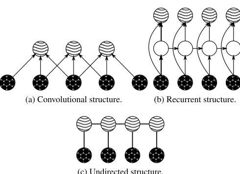
(a) Convolutional structure. (b) Recurrent structure.
(c) Undirected structure.
Figure 1: The two model structures that are used in this paper. The wavy circles represent the hidden units, the circles filled with dots the visible units and empty circles represent deterministic functions. The time dimension runs from the left to the right and each circle represents a layer of units.
3. The Recurrent Energy-Based Model
The second model we propose in this paper is the Recurrent Energy-Based Model (REBM). In this model, the energy is based on the dynamics that the data elicit in a non-linear dynamical system. In this case the non-linear dynamical system is instantiated as a Recurrent Neural Network (RNN).
RNNs are interesting models for time-series because they can process sequences of arbitrary length. Unlike Hidden Markov Models, RNNs have hidden states that are high dimensional dis-tributed representations of the previous input patterns.
The energy function of the REBM is again defined by Equation 3 butgconvis replaced by grec(V,t;θRNN) =Axt+Bvt+br,
xt=tanh(Cxt−1+Dvt+bx) 1<t≤T,
whereA,B,CandDare matrices with network connection parameters andbrandbxare the bias vectors of, respectively, the output variables and the hidden state variables X. The total set of trainable parameters for this model is given byθ={bh} ∪θRNNwithθRNN={A,B,C,D,br,bx}. See Fig. 1b for a graphical representation of the recurrent architecture.
In most situations, predictions by an RNN only depend on the previous input patterns. For the REBM however, the energy function depends on the full input sequence. This allows predictions to be based on future observations as well.
4. The Discriminative Temporal Boltzmann Machine
The third model is inspired by the work on Deep Boltzmann Machines (Salakhutdinov and Hinton, 2009) and variational inference. In this model, the hidden units are connected over time in a way that is similar to an undirected version of the factorial Hidden Markov Model (Ghahramani and Jordan, 1997). Unlike the factorial Hidden Markov Model however, the hidden variables are not just connected in temporal chains that would be independent given the input (note that this statement is only true for undirected graphs). In this model, every hidden unit at a certain time step t is connected to every hidden unit at timet+1 and timet−1. This allows the model to use distributed representations that are highly interconnected. The hidden units are again binary and take values from{−1,1}. The energy of the model is defined by the following equation:
E(V,H) =
T
∑
t=1
kvt−bvk2 2σ2 −h
T
t−1Wht−hTt Avt−htTbh
,
whereh0 is defined to be 0. Note that this energy function is very similar to Equation 3, but the convolution has been replaced with a matrix multiplication and there is an additional term that parametrizes correlations between hidden units at adjacent time steps. The structure of the model is shown in Fig. 1c. This model can also be seen as a Deep Boltzmann Machine in which every layer is connected to a different time step of the input sequence. Because this model has the structure of a Boltzmann Machine time-series model and will be trained in a discriminative way, we will refer to the model as the Discriminative Temporal Boltzmann Machine (DTBM). This model is very similar to the one proposed in Williams and Hinton (1991) for discrete data but the way in which we will train it is very different.
4.1 Inference
Since the hidden units of the DTBM are not independent from each other, we are not able to use the free energy formulation from Equation 4. Even when values of the visible units are all known, inference for the hidden units is still intractable. For this reason, we use variational mean-field to minimize the free energy. Compared to other approximate inference algorithms like loopy belief propagation, variational mean-field is relatively computationally efficient as the number of messages to compute is equal to the number of variables rather than their pairwise interactions. In the DTBM the number of pairwise interactions is very large compared to the actual number of variables.
In the original training procedure for the Deep Boltzmann Machine (Salakhutdinov and Hinton, 2009), the free energy is replaced by a variational lower-bound on the log likelihood. Given a set of known variablesxand a set of unknown variablesy, this bound can be written as
lnp(x)≥
∑
y
q(y|x;u)lnp(x,y) +
H
(q),whereq(·)is an approximating distribution with parametersuand
H
(·)is the entropy functional. If the approximating distribution is chosen to be a fully factorized Bernoulli distribution of the form∏tT=1∏Nhj=1q(hjt|ujt), withq(hjt =1|ujt) = 12(ujt+1), q(hjt=−1|ujt) = 12(1−ujt) andNh the number of hidden units, a simple algorithm can be derived that optimizes the setU∈(0,1)Nh×T
of variational parameters to maximize the bound. While the Deep Boltzmann Machine is originally trained by approximating the free energy component of the gradient with the variational method and the term of the gradient that comes from the partition function with sampling methods, we will only use the variational optimization as our inference algorithm.
Because the distribution will now also be defined over some of the visible units that have been labelled as missing, the variational distribution is augmented with the appropriate number of one-dimensional Gaussian distributions of unit variance of the form q(v|uˆ) =
N
(v|uˆ,1). The lower bound now has the following form:lnp(V\Ω)≥
B
(U¯) =T
∑
t=1
−kvt−bvk 2 \Ω
2σ2 +u T
t−1Wut+uTt bh
−kˆut−bvk 2
Ω
2σ2 +
∑
k,i∈ΩAkiuktuˆit+
∑
k,i6∈ΩAkiuktvit
− Nh
∑
j=1
ujt+1 2 ln
ujt+1
2 +
1−ujt 2 ln
1−ujt 2
!
+1
2Nuˆln(2πeσ
2)−lnZ(θ),
whereΩis the set of indices that point to the variables that have been labelled as missing,Nuˆis the number of Gaussian variables to predict (i.e., the number of missing values) andU¯ is the set of all mean field parametersU∪Uˆ. Note that an upper bound on the free energy is now defined as
E(V\Ω)≤ −
B
(U¯)−lnZ(θ).Optimizing this bound will lead to values of the variational parameters that approach a mode of the distribution in a similar way that a minimization of the free energy by means of gradient descent will. Setting the gradient of this bound with respect to the mean-field parameters to zero, leads to the following update equations:
ut ←tanh(WTut+1+Wut−1+bh+A ˆut), (5)
ˆut ←bv+ATut. (6)
Note that only the variables ˆuthat correspond to missing values get updated.
is guaranteed to converge to a local minimum of the free energy surface because every individual update achieves the unique minimum for that update and the updates are linearly independent.
The model will be trained to make the variational inference updates more efficient for imputa-tion. The naive mean-field iterations will approach a local mode of the distribution and the values of the parameters ˆucan be directly interpreted as predictions. Note that Salakhutdinov and Larochelle (2010) proposed a method that hints in this direction by training a separate model to initialize the mean-field algorithm as well as possible.
5. Computing Loss Gradients
To train the models above, it is necessary to compute the gradient of the loss function with respect to the parameters. The loss gradients of both the models that use gradient descent inference can be computed in a similar way. For these models, only the gradient of the energy is different. Since the DTBM uses a different inference procedure, we describe the computation of its loss gradient in a separate subsection.
5.1 Backpropagation Through Gradient Descent
To train the models that use gradient descent inference (i.e., the convolutional and recurrent models), we backpropagated loss gradients through the gradient descent steps like in Domke (2011). Given an input pattern and a set of indices that point to the missing values, a prediction was first obtained by doingKsteps of gradient descent with step sizeλon the free energy. Subsequently, the gradient of the mean squared error lossLwith respect to the parameters was computed by propagating errors back through the gradient descent steps in holder variables V¯ andθ¯ that in the end contained the gradient of the error with respect to the input variables and the parameters of the models (we useθ as a place holder for both the biases and weights of the models). Note that this procedure is similar to the backpropagation through time procedure for recurrent neural networks. The gradient with respect to the parameters was used to train the models with stochastic gradient descent. Hence, the models were trained to improve the predictions that the optimization procedure came up with directly.
Backpropagation is an application of the chain rule to propagate the error gradient back to the parameters of interest by multiplication of a series of derivatives. A single gradient descent inference step over the input variables is given by
ˆ
Vk+1←Vˆk−λ∇VE(Vˆk;θ). (7) By application of the chain rule, the gradient of the loss with respect to the parametersθis given by
∂L
∂θ = K
∑
k=1 ∂L
∂Vˆk ∂Vˆk
∂θ . (8)
Assuming a value ofkthat is smaller thanK−1 the gradient of the loss with respect to one of the intermediate states of the variablesVˆkis given by
∂L
∂Vˆk = ∂L
∂VˆK ∂VˆK
∂VˆK−1· · · ∂Vˆk+1
To propagate errors back we need to know∂Vˆk+1/∂Vˆk. Differentiating Equation 7 with respect to Vgives
∂Vˆk+1
∂Vˆk =I−λ
∂2E(Vˆk;θ) ∂V∂VT .
Similarly, to complete the computation in Equation 8, we also need to know∂Vˆk+1/∂θto propagate the errors back to the model parameters. This partial derivative is given by
∂Vˆk+1 ∂θ =−λ
∂2E(Vˆk;θ) ∂θ∂VT .
Since we are using gradients of gradients, we need to compute second order derivatives. Both of these second order derivatives are matrices that contain a very large number of values but fortu-nately there are methods to compute their product with an arbitrary vector efficiently (Domke, 2012; Pearlmutter, 1994). It is never required to explicitly store these values.
One way to compute the product of the second order derivative with a vector is by finite differ-ences using
df
dyTv≈ 1
2ε(f(y+εv)−f(y−εv)).
The error of this approximation is
O
(ε2). Another way to compute these values is by means of automated differentiation or theR
operator (Pearlmutter, 1994). In software for automated dif-ferentiation like Theano (Bergstra et al., 2010), the required products can be computed relatively efficiently by taking the inner product of the gradient of the energy with respect to the input and the vector to obtain a new cost value. The automated differentiation software can now be used to differentiate this new function again with respect to the input and the parameters.We found that, even when applied recursively for three steps in single precision, the finite dif-ferences approximation was very accurate. For the CEBM, the mean squared difference between the finite differences based loss gradients and the exact gradients was of order 10−3, while the vari-ance of the gradients was of order 102. In preliminary experiments, we didn’t see any effect of the approximation on the actual performance for this model.
Since the finite difference approximation was generally faster than the exact computation of the second order derivatives, we used it for most of the required quantities. For the REBM we used finite differences withε=10−7in double precision. For the CEBM we found that automatic differentiation for the second order derivative with respect to the parameters was faster so for this quantity we used this method instead of finite differences. The CEBM computations were done on a GPU so we had to use single precision withε=10−4.
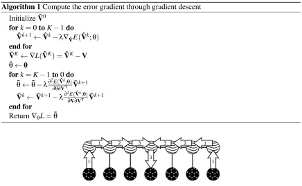
See Algorithm 1 for more details about the backpropagation through gradient descent procedure. In the algorithm we omitted that all references to the data only concern the missing values to avoid overly complicated notation.
5.2 Backpropagation Through Mean-Field
Computing error gradients for the mean-field based model is possible by backpropagating errors through the mean-field updates. Intuitively, this model can be seen as a bi-directional recurrent neural network with tied weights. The derivatives of the update Equations 5 and 6 are easy to compute using the derivatives of the hyperbolic tangent function and linear operations:
∂tanh(Wz)
∂z =W
Algorithm 1Compute the error gradient through gradient descent
InitializeVˆ0
fork=0toK−1do ˆ
Vk+1←Vˆk−λ∇VˆE(Vˆk;θ)
end for ¯
VK←∇L(VˆK) =VˆK−V ¯
θ←0
fork=K−1to0do ¯
θ←θ¯−λ∂2E(Vˆk;θ)
∂θ∂VT V¯k+1
¯
Vk←V¯k+1−λ∂2E(Vˆk;θ)
∂V∂VT V¯k+1
end for
Return∇θL=θ¯
✁ ✂ ✂ ✁
✂
Figure 2: Flow of information due to mean-field updates. The numbers represent the separate itera-tions at which both the hidden units and the unknown visible units are updated.
However, to make it easy to experiment with the number of mean-field iterations, we used automated differentiation for this.
While the number of gradient descent steps for the convolutional model and the recurrent neural network model can be very low, the number of mean-field iterations has a more profound influence on the behavior of the model. This is because the number of mean-field iterations directly deter-mines the amount of context information that is available to guide the prediction of the missing values. If for example, five iterations of mean-field are used, the activation in the hidden variables at a certain time frameht will be influenced by the five frames of visible variables to the left and right of it and by the known values ofvt; every vector of hidden units now depends on eleven frames of visible units. So a greater number of mean-field iterations increases the range of the dependencies the model can capture. This flow of information is displayed for three iterations in Fig. 2.
Using backpropagation through variational optimization updates is referred to as variational mode learning (Tappen, 2007). In Tappen (2007), Fields of Experts were trained by backpropagating loss function gradients through variational updates that minimized a quadratic upper bound of the loss function. This specific approach would not work for the type of model we defined here.
6. Experiments
To compare our approach with generative methods, we also trained a Convolutional RBM with the same energy function as the Convolutional Energy-Based Model all these data sets. Between these two models, the training method is the only thing that makes them different. Furthermore, we also trained a Recurrent Neural Network Restricted Boltzmann Machine (RNN-RBM; Boulanger-Lewandowski et al. 2012). This model is quite similar to the REBM as it also employs separate sets of deterministic recurrent units and stochastic hidden units. The structure of the RNN-RBM is the same as the architecture in Fig. 1b but the hidden units are connected to the next time step instead of the current one and those connections are undirected. This makes it possible to use Contrastive Divergence learning but also renders the model unable to incorporate future information during inference because the information from the recurrent units is considered to be fixed. Training a recurrent model that incorporates this kind of information with Contrastive Divergence would require something like Hybrid Monte Carlo (Duane et al., 1987). Unfortunately, Hybrid Monte Carlo requires careful tuning of the number and size of leap frog steps and is known to be less efficient than block Gibbs sampling.
For the Energy-Based models we used the same inference procedure as during training. For the Convolutional RBM and RNN-RBM we used mean-field iterations that were run until the MSE changed less than a threshold of 10−5. For the RNN-RBM this was done by initializing the missing values of a single time step with the values of the corresponding dimensions at the previous time-step, running mean-field to update them, passing these new values through the recurrent neural network and repeating this procedure for all remaining time-steps. This procedure proved to be more accurate than Gibbs sampling which was originally used to generate sequences with this model (Boulanger-Lewandowski et al., 2012).
6.1 Concatenated Handwritten Digits
To provide a qualitative assessment of the reconstruction abilities of the models, we used the USPS handwritten digits data set (http://www.cs.nyu.edu/˜roweis/data/usps_all.mat). While the task we trained the models on is of little practical use, visual inspection of the reconstructions allows for an evaluation of the results that may be more insightful than just the mean squared error with respect to the ground truth.
6.1.1 DATA
The USPS digits data set contains 8-bit grayscale 28×28 pixel images of the numbers ‘0’ through ‘9’. Each class has 1100 examples. To turn the data into a time-series task, we randomly permuted the order of the digits and concatenated them horizontally. This sequence of 28 dimensional vectors was split into a train set, a validation set and a test set that consisted of respectively 80% and two times 10% of the data.
6.1.2 TRAINING
Good settings of the hyper parameters of the models were found with a random search2 over 500 points in the parameter space, followed by some manual fine-tuning to find the settings that led to minimal error on the validation set. After this, the models were trained again on both the train
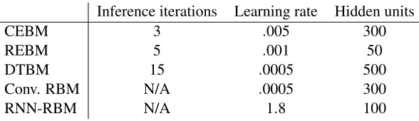
Inference iterations Learning rate Hidden units
CEBM 3 .005 300
REBM 5 .001 50
DTBM 15 .0005 500
Conv. RBM N/A .0005 300
RNN-RBM N/A 1.8 100
Table 1: Parameter settings for training the models on the USPS data. The learning rates were always divided by the lengths of the sequences during training.
and the validation data with these settings. Since the CEBM, DTBM and Convolutional RBM are very parallel in nature, we used a GPU for their simulations. All models were trained for 100,000 epochs on randomly selected mini batches of 100 frames. Linearly decaying learning rates were used. Table 1 shows the settings of the hyper parameters. After some preliminary experimentation we found that we got better results for the CEBM by initializing the biases of the hidden units at -2 to promote sparsity. We used a step size of.03 for the gradient descent inference algorithm of the CEBM. The REBM had 200 recurrent units and we used a step size of.2 for the gradient descent inference. The CEBM and the Convolutional RBM had a window size of 7 time frames. The RNN-RBM had 200 recurrent units. Note that the best RNN-RNN-RBMs also had more hidden units than the best performing REBMs.
The Convolutional RBM was trained with the Contrastive Divergence algorithm (CD; Hinton 2002). We found that we got better results with this model if we increased the number of CD sampling steps over time. Initially a single CD step was used. After 20,000 iterations this number was increased to 5, after 50,000 to 10 and after 75,000 to 20. We did not find any benefits from stimulating sparsity in this model. For the RNN-RBM we found that a fixed number of 5 CD sampling steps gave the best results.
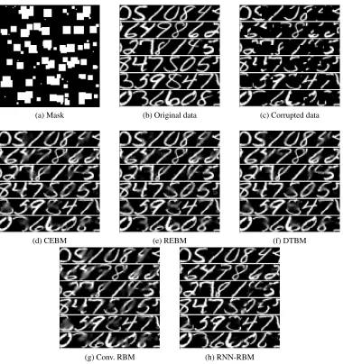
Missing values were generated as 20 square shaped gaps in every data sequence. The gaps were positioned at uniformly sampled locations. The size of each square was uniformly sampled from the set{1,2, . . . ,8}. Fig. 3a shows an example of missing values that were generated this way for six sequences. Fig. 3c shows an example of data that has been corrupted by this pattern of missing values.
For this experiment, the Energy-Based Models that required missing values during training were provided with missing values from the same distribution that was used to select them for evaluation. To control for the random initialization of the parameters and the randomness induced by stochastic gradient descent, we repeated every experiment 10 times.
6.1.3 RESULTS
Train Test CEBM .48(.0082) .49(.0089)
REBM .47(.01) .48(.0067)
DTBM .44(.011) .45(.0088)
Conv. RBM .66(.011) .66(.0085)
RNN-RBM .71(.0056) .73(.0062)
Table 2: Means and standard deviations of the results in mean squared error on the USPS data.
(a) Mask (b) Original data (c) Corrupted data
(d) CEBM (e) REBM (f) DTBM
(g) Conv. RBM (h) RNN-RBM
of these models are similar. The DTBM provided reconstructions that look similar in quality to those of the REBM. The RNN-RBM has a very bad MSE score while its reconstructions look very sharp when they are correct. Somehow, this model seems to be too sure in cases where it is not able to fill in the data well. This may be due to the fact that the reconstructions are generated on a frame-by frame basis while the deterministic models and the Convolutional RBM can update their predictions from previous iterations. This causes bad predictions to be propagated and possibly amplified. Unfortunately this problem is intrinsic to the choice to keep sampling tractable by treating the recurrent mapping as fixed context information.
6.2 Motion Capture
For the second experiment we applied the models to a motion capture data set. In visual motion capture, a camera records movements of a person wearing a special suit with bright markers attached to it. These markers are later used to link the movements to a skeleton model. Missing values can occur due to lightning effects or occlusion. Motion capture data is high dimensional and generated by a non-linear process. This makes motion capture reconstruction an interesting task for evaluating more complex models for missing value imputation.
In previous work (Taylor et al., 2007), a Conditional Restricted Boltzmann Machine (CRBM) was trained to impute missing values in motion capture as well. For comparison we also train a CRBM but note that a direct comparison of performance is not fair because the CRBM only uses information from a fixed number of previous frames to make predictions.
6.2.1 DATA
The data consisted of three motion capture recordings from 17 marker positions represented as three 49-dimensional sequences of joint angles. The data was down sampled to 30Hz and the sequences consisted of 3128, 438, and 260 frames. The first sequence was used for training, the second for validation and the third for testing. The sequences were derived from a subject who was walking and turning and come from the MIT data set provided by Eugene Hsu.3 The data was preprocessed by Graham Taylor (Taylor et al., 2007) using parts of Neil Lawrence’s Motion Capture Toolbox.
6.2.2 TRAINING
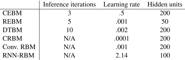
Again, good settings of the hyper parameters of the models were found with a random search on the parameter space, followed by some manual fine-tuning to find the settings that led to minimal error on the validation set. The models were trained on mini batches of 140 frames. Table 3 shows the hyper parameter settings of the models. Note that the best RNN-RBMs had again more hidden units than the best REBMs. Additionally, the inference step sizes of the CEBM and the REBM were both set to.2. The CEBM and the Convolutional RBM had a window size of 15 time frames. All models were trained for 50,000 iterations. The REBM had 200 recurrent units. To train the Convolutional RBM, single iteration CD training was used during the first 10,000 epochs. Five iterations of CD were used during the remaining training epochs. The CRBM was trained with single iteration CD. Finally, the RNN-RBM had 200 recurrent units and was trained with 5 CD iterations. All models were trained for a total of 50,000 epochs.
Inference iterations Learning rate Hidden units
CEBM 3 .5 200
REBM 5 .001 50
DTBM 10 .002 200
CRBM N/A .0001 200
Conv. RBM N/A .001 200
RNN-RBM N/A 2.14 100
Table 3: Parameter settings for training the models on the motion capture data. The learning rate values were divided by the lengths of the sequences during training.
The CEBM, REBM and DTBM were again trained by labeling random sets of dimensions as missing. The number of missing dimensions was sampled uniformly. The specific dimensions were then randomly selected without replacement. The duration of the data loss was sampled uniformly between 60 and 125 frames. This adds some bias towards situations in which the same dimensions are missing for a certain duration. This seems to be a sensible assumption in the case of motion capture data and it is an advantage of the training method that it is possible to add this kind of in-formation. To control for the influence of the randomly initialization of the parameters, we repeated every experiment 10 times.
Finally, Nearest neighbour interpolation was done by selecting the frame from the train set with minimal Euclidean distance to the test frame according to the observed dimensions. The distances were computed in the normalized joint angle space.
6.2.3 EVALUATION
To evaluate the models, a set of dimensions was removed from the test data for a duration of 120 frames (4 seconds). This was done for either the markers of the left leg or the markers of the whole upper body (everything above the hip). Because the offset of this gap was chosen randomly and because the CRBM had a stochastic inference procedure, this process was repeated 500 times to obtain average mean squared error values for both the train and the test data. Note that this distribution of missing values was quite different from the one that was used during training.
The CRBM was used in a generative way by conditioning it on the samples it generated at the previous time steps while clamping the observed values and only sampling those that were missing as was done the work by Taylor et al. (2007). Preliminary results showed that this led to similar results to the use of mean-field or minimization of the model’s free energy to do inference.
6.2.4 RESULTS
Left leg Upper body
Train Test Train Test
CEBM .18(.0036) .29(.011) .47(.023) .46(.017)
REBM .22(.0047) .33(.017) .47(.014) .42(.014)
DTBM .17(.0069) .28(.017) .43(.021) .45(.011)
CRBM .25(.0036) .44(.014) .51(.023) .49(.0065)
Conv. RBM .16(.0038) .36(.027) .48(.015) .68(.035)
RNN-RBM .18(.0055) .36(.023) .45(.017) .60(.055)
Nearest neighb. N/A .45 N/A .76
Table 4: Means and standard deviations of the results in mean squared error on the motion capture data.
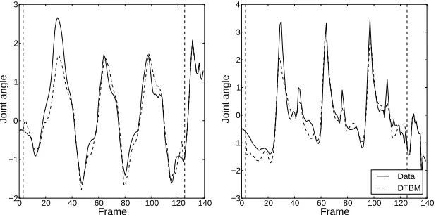
Figure 4: Plots of two dimensions reconstructed by the DTBM next to the actual data. For this sequence the markers of the left leg were missing in the region between the vertical striped lines.
when reconstructing the markers of the missing leg. It performed slightly better at reconstructing the missing upper body than the Convolutional RBM but still a lot worse than the three deterministic models. Fig. 4 shows plots of the predictions made by the DTBM for two of the markers for a sequence from the test data.
6.3 Missing Training Data
Inference iterations Learning rate Hidden units
CEBM 3 .65 300
REBM 3 .0007 100
DTBM 5 .002 300
Conv. RBM N/A .00012 300
RNN-RBM N/A .15 50
Table 5: Parameter settings for training the models on the robot data. The learning rates were always divided by the lengths of the sequences during training.
artificially created missing values for which the ground truth is known. A very similar method has been used in earlier work to train neural networks for classification when missing values are present (Bengio and Gingras, 1996).
To see how well our models deal with missing training data, we conducted an additional series of experiments.
6.3.1 DATA
The data we used to investigate the effect of missing training data consists of the measurements of the 24 ultrasound sensors of a SCITOS G5 robot navigating a room (Freire et al., 2009; Frank and Asuncion, 2010). The 5456 sensor readings were sampled at a rate of 9Hz and the robot was following the wall of the room in a clockwise direction, making four trips around the room. We used 80% of the data for training and split the remaining 20% up in a validation set and a test set.
6.3.2 TRAINING
In the first experiment, we trained the models on fully intact training data to get an estimate of the optimal performance the models could achieve on it. In this experiment we also compare the results with those of the Convolutional RBM and the RNN-RBM. In the second experiment, we generated a mask for the whole train set. The mask was divided in regions of 100 frames and at each of these regions a randomly selected set of dimensions was labelled as missing. To train the models, we selected random batches of 100 frames from the train data and selected another set of variables as missing that were not already truly missing in the data. This way, the models never had access to the values that were labelled as missing by the training data mask. To investigate the robustness of the models, we varied the amount of data that was damaged in the train set. In both experiments, the number of dimensions that we pretended to be missing in order to train the models was uniformly sampled from{1, . . . ,5}. All models were trained for 100,000 epochs.
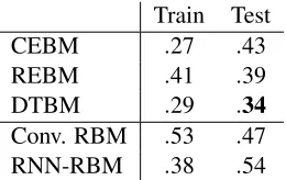
Train Test CEBM .27 .43 REBM .41 .39 DTBM .29 .34
Conv. RBM .53 .47 RNN-RBM .38 .54
Table 6: Results in mean squared error on the wall robot data without missing dimensions during training.
Figure 5: Mean square error as a function of the number of missing dimensions in the train data.
6.3.3 RESULTS
Table 6 shows the results for the experiment without missing train data. The DTBM had the best performance, followed by the REBM, the CEBM, the Convolutional RBM, and the RNN-RBM respectively. Surprisingly, the CEBM has a far better score on the train data than the REBM while its test error is higher. This seems to be a sign of overfitting. The REBM is probably slightly underfitting as its training error was even a little bit higher than its test error. The RNN-RBM obtained a slightly better score on the train data than the REBM but performed a lot worse on the test set.
Fig. 5 shows the error scores for the three energy-based models as a function of the number of missing input dimensions. Obviously, as more dimensions are missing, there is less data available to train on and the error scores of all the models are rising. For the DTBM and REBM, the error seems to increase at a modest pace initially and when just a single value is missing, the performance is similar to the first experiment. The CEBM has more trouble with missing values and is not learning to reconstruct the data well any more after about 10 dimensions are missing. We interpret these results as an upper bound on the error scores one could potentially achieve by doing more extensive hyper parameter tuning for each individual level of data corruption.
7. Discussion
Convolu-tional RBM. This indicates that our training strategy is more suited for missing value imputation than the Contrastive Divergence algorithm. The REBM also outperformed the RNN-RBM. While this comparison is less valid because the two models are not entirely the same, it still suggests that our training method also works better for recurrent architectures. The DTBM outperformed all other methods in all of the experiments except for reconstructing the upper body markers of the motion capture data set where the REBM performed better. Given that it is also the easiest model to imple-ment and relatively computationally efficient compared to the other models, this model seems to be the most promising candidate for practical applications.
We didn’t show that our method outperforms maximum likelihood learning because Contrastive Divergence is not optimizing the actual likelihood of the model. However, it seems to be the most popular method for training these kind of models when true maximum likelihood learning is in-tractable. We actually suspect that, compared to other approximate maximum likelihood methods, Contrastive Divergence is still one of the best candidates for missing value imputation because it optimizes the energy landscape locally by pushing up wrong predictions that are near the data itself. When the number of missing values is not too large, inference would start near one of the regions in which the energy landscape has a shape that promotes good predictions. When the number of missing values is too high however, the inference algorithm might start in a region that was not explicitly shaped by the learning algorithm because it was too far away from the data. This might explain the bad performance of the Convolutional RBM when the whole upper body was missing in the motion capture task. The CRBM and (to a lesser extent) the RNN-RBM were more robust in this situation.
7.1 Relation to Other Models
As mentioned before, our training algorithm is based on the work by Domke (2011) with the main difference that we optimize a loss function that only considers a subset of the data variables. Ex-cept for the CEBM, our models also have a far more complicated structure and we think that the discriminative training methods are not just more computationally efficient but actually allow us to train models that would otherwise be very difficult to train at all.
Our work is also related to the training of Dynamical Factor Graphs (DFG; Mirowski and LeCun 2009). DFGs are used as generative models, but the way they are trained is more similar to the energy-based learning framework. The types of DFGs that have been studied so far are similar to our REBM model in that they employ both recurrent connections and latent variables. An important difference is that in the REBM the latent variables are not involved in the recurrent part of the model. By constraining the latent states of a DFG to operate under Gaussian noise with fixed covariance, the partition function of the model becomes constant so that a minimization of the energy for a certain state will automatically push up the energy values of all other possible states. The model is not fully probabilistic as it aims to align its maximum a posteriori hidden states with the observed data instead of the sum over all their possible values.
Inference for missing values in DFGs is done with gradient descent to find the minimum energy latent state sequence, ignoring the missing values in the gradient computations. Subsequently, the missing values are predicted as a function of this latent state sequence. There are a couple of important differences with our approach:
• The CEBM and REBM models use only a limited number of gradient descent updates while for DFGs this minimization is run until convergence.
• In the CEBM and REBM, energy minimization only takes place with respect to the missing values and not with respect to the latent variables which are marginalized out analytically.
It seems that some of the ideas behind DFGs are orthogonal to our approaches and may be combined to design new interesting models.
Recently, a generative model called NADE (Larochelle and Murray, 2011) was proposed in which the mean-field algorithm inspired a model similar to the Restricted Boltzmann Machine (Fre-und and Haussler, 1994; Hinton, 2002), but with a tractable inference algorithm. In this model, a single iteration of mean-field is used to approximate a set of conditional distributions that are com-bined into a generative model. Our mean-field based model is substantially different in that it doesn’t try to learn a joint distribution over all the variables and that mean-field is also used to estimate the influence of connections between the hidden variables. NADE has been combined with a recurrent neural network to construct a sequential model for note patterns in music (Boulanger-Lewandowski et al., 2012). This model is practically the same as the RNN-RBM we used as a baseline but with the RBM replaced by the NADE model. To our knowledge, NADE has not been applied to continu-ous data yet, unlike the Recurrent Temporal Restricted Boltzmann Machine (Sutskever et al., 2008), which is more similar to the RNN-RBM.
Adding artificial corruption to the data and training a model to reconstruct it is similar to the way denoising autoencoders are trained (Vincent et al., 2008). The most important difference is that our models only focus on recovery of the missing values given the observed variables and not on reconstructing both.
The way the DTBM model dealt with missing training data in Section 6.3, is very similar to a method for dealing with missing values in neural networks that was presented more than a decade ago (Bengio and Gingras, 1996). In this method, missing values are also filled in by updating them as if they are part of a recurrent neural network. An important difference with our work is that in the work by Bengio and Gingras (1996) the goal was not to predict the missing values themselves, but to perform better on classification tasks when missing values in the inputs are present.
It turns out that the architecture of the DTBM has also been proposed for learning to discriminate between sequences (Williams and Hinton, 1991). In this work, a version of the mean field algorithm that is inspired by simulated annealing is ran until convergence and the training algorithm aims to maximize the lower bound on the likelihood for one class of sequences, while lowering it for the remaining classes. Running mean-field iterations until convergence can make training very inefficient so it might be interesting to see how backpropagation through mean-field performs for tasks of this type.
7.2 Limitations
Another downside of our approach is that it introduces new hyper parameters to tune. These are the number of inference iterations and for the CEBM and the REBM also the step size of the gradient descent algorithm. Because of this, we found it easier to find good settings for the DTBM than for the CEBM and REBM. This problem could be solved to some extent by using an optimizer for inference in the CEBM and the REBM that doesn’t need a step size parameter. LBFGS has been shown to work quite well for optimization based inference (Domke, 2011) but is a lot more complicated to implement.
The REBM was the most difficult model to train even though it sometimes performed better than the CEBM. It seems to be more sensitive to the initial hyper parameter settings than the other models. As more hidden units were used, these models became more difficult to optimize and this explains why the optimal number of hidden units was generally lower than for the other models. We think this problem occurs because the energy gradient is computed with backpropagation through time over relatively long sequences. The gradients of recurrent neural networks are known to be prone to exponential growth or decay and a single bad gradient can lead to a divergence of the learning algorithm. Larger numbers of hidden units tend to lead to larger values in the gradients, making problematic weight updates more frequent. In preliminary results we found that this prob-lem can be solved to some extent by normalizing the loss gradient before updating the weights. The DTBM might suffer less from this problem because the number of backpropagation steps that are used is smaller.
Since the number of mean-field iterations of the DTBM is directly related to the length of the temporal dependencies it can model, it might not be very suitable for problems in which these dependencies are very long. That being said, this model benefits a lot from parallel computing machinery like GPUs. As the performance of parallel computing hardware increases, the compu-tational time required to model dependencies that are as long as the sequence itself might become more comparable to simulating a regular recurrent neural network. It remains to be seen what kind of effect this has on the quality of the computed gradients.
7.3 Conclusion
We presented a strategy for training models for missing value imputation in high dimensional time-series. The three models we proposed showed promising performance on concatenated digits in-painting, missing marker restoration for motion capture and imputation of values for robot sensors. Our training methods appear to be more suitable for missing value imputation than Contrastive Di-vergence learning, given similar model architectures. Furthermore, the models could also handle missing values in the training data itself and seem to be relatively robust to these corruptions.
Future work should investigate the performance of different inference methods. Interesting candidates would be variants of loopy belief propagation, expectation propagation and structured mean-field. It would also be interesting to see if models of this type can be designed for other task domains like image inpainting.
Acknowledgments
References
A. Barbu. Training an active random field for real-time image denoising. IEEE Transactions on
Image Processing, 18(11):2451–2462, 2009.
Y. Bengio and F. Gingras. Recurrent neural networks for missing or asynchronous data. Advances
in Neural Information Processing Systems, pages 395–401, 1996.
J. Bergstra, O. Breuleux, F. Bastien, P. Lamblin, R. Pascanu, G. Desjardins, J. Turian, D. Warde-Farley, and Y. Bengio. Theano: A CPU and GPU math compiler in python. In S. van der Walt and J. Millman, editors,Proceedings of the 9th Python in Science Conference, pages 3–10, 2010.
M. Bertalm´ıo, G. Sapiro, V. Caselles, and C. Ballester. Image inpainting. InSIGGRAPH, pages 417–424, 2000.
D. P. Bertsekas. Nonlinear Programming. Athena Scientific, Belmont, MA, 1999.
C. M. Bishop.Pattern Recognition and Machine Learning. Springer-Verlag New York, Inc., Secau-cus, NJ, USA, 2006. ISBN 0387310738.
N. Boulanger-Lewandowski, Y. Bengio, and P. Vincent. Modeling temporal dependencies in high-dimensional sequences: Application to polyphonic music generation and transcription. In
Pro-ceedings of the 29th International Conference on Machine Learning. Omnipress, 2012.
P. Brakel, S. Dieleman, and B. Schrauwen. Training restricted Boltzmann machines with multi-tempering: Harnessing parallelization. In A. E. P. Villa, W. Duch, P. ´Erdi, F. Masulli, and G. Palm, editors,ICANN (2), volume 7553 ofLecture Notes in Computer Science, pages 92–99. Springer, 2012. ISBN 978-3-642-33265-4.
G. Desjardins, A. C. Courville, Y. Bengio, P. Vincent, and O. Delalleau. Tempered Markov chain Monte Carlo for training of restricted boltzmann machines. InProceedings of the International Conference on Artificial Intelligence and Statistics, pages 145–152, 2010.
J. Domke. Parameter learning with truncated message-passing. In Proceedings of the 2011
IEEE Conference on Computer Vision and Pattern Recognition, CVPR ’11, pages 2937–2943,
Washington, DC, USA, 2011. IEEE Computer Society. ISBN 978-1-4577-0394-2. doi: 10.1109/CVPR.2011.5995320.
J. Domke. Generic methods for optimization-based modeling. InProceedings of the International Conference on Artificial Intelligence and Statistics, pages 318–326, 2012.
S. Duane, A. D. Kennedy, B. J. Pendleton, and D. Roweth. Hybrid monte carlo. Physics Letters B, 195(2):216–222, 1987.
A. Frank and A. Asuncion. UCI machine learning repository, 2010. URLhttp://archive.ics. uci.edu/ml.
Y. Freund and D. Haussler. Unsupervised learning of distributions on binary vectors using two layer networks. Technical report, Santa Cruz, CA, USA, 1994.
Z. Ghahramani and M. I. Jordan. Factorial hidden markov models. Machine Learning, 29(2-3): 245–273, 1997.
Z. Ghahramani and S. T. Roweis. Learning nonlinear dynamical systems using an EM algorithm.
InAdvances in Neural Information Processing Systems, pages 599–605. MIT Press, 1999.
A. Gupta and M. S. Lam. Estimating missing values using neural networks. Journal of the Opera-tional Research Society, pages 229–238, 1996.
G. E. Hinton. Training products of experts by minimizing contrastive divergence. Neural Compu-tation, 14(8):1771–1800, 2002.
G. E. Hinton, S. Osindero, and Y. W. Teh. A fast learning algorithm for deep belief nets. Neural
Computation, 18(7):1527–1554, 2006.
A. Hyv¨arinen. Estimation of non-normalized statistical models by score matching. Journal of
Machine Learning Research, 6:695–709, 2005.
V. Jain, J. F. Murray, F. Roth, S. C. Turaga, V. P. Zhigulin, K. L. Briggman, M. Helmstaedter, W. Denk, and H. S. Seung. Supervised learning of image restoration with convolutional networks. InICCV, pages 1–8. IEEE, 2007.
D. Koller and N. Friedman. Probabilistic Graphical Models: Principles and Techniques. MIT Press, 2009.
H. Larochelle and I. Murray. The neural autoregressive distribution estimator. JMLR: W&CP, 15: 29–37, 2011.
N. D. Lawrence. Gaussian process latent variable models for visualisation of high dimensional data. In S. Thrun, L. K. Saul, and B. Sch¨olkopf, editors,Advances in Neural Information Processing
Systems. MIT Press, 2003. ISBN 0-262-20152-6.
N. D. Lawrence. Learning for larger datasets with the gaussian process latent variable model. In
Proceedings of the Eleventh International Conference on Artificial Intelligence and Statistics, pages 21–24. Omnipress, 2007.
Y. LeCun and F. Huang. Loss functions for discriminative training of energy-based models. In
Proceedings of the 10-th International Conference on Artificial Intelligence and Statistics, 2005.
Y. LeCun, S. Chopra, R. Hadsell, M. Ranzato, and F. Huang. A tutorial on energy-based learning. In G. Bakir, T. Hofman, B. Sch¨olkopf, A. Smola, and B. Taskar, editors, Predicting Structured Data. MIT Press, 2006.
H. Lee, R. Grosse, R. Ranganath, and A. Y. Ng. Convolutional deep belief networks for scalable unsupervised learning of hierarchical representations. In Proceedings of the 26th Annual
Inter-national Conference on Machine Learning, pages 609–616, New York, NY, USA, 2009. ACM.
P. Mirowski and Y. LeCun. Dynamic factor graphs for time series modeling. InProceedings of the
European Conference on Machine Learning, 2009.
F. V. Nelwamondo, S. Mohamed, and T. Marwala. Missing data: A comparison of neural network and expectation maximisation techniques. arXiv pre-print, 2007.
J. Pearl. Probabilistic Reasoning in Intelligent Systems: Networks of Plausible Inference. Morgan Kaufmann Publishers Inc., San Francisco, CA, USA, 1988. ISBN 0-934613-73-7.
B. A. Pearlmutter. Fast exact multiplication by the Hessian.Neural Computation, 6:147–160, 1994.
B. Polyak. Some methods of speeding up the convergence of iteration methods. USSR
Computa-tional Mathematics and Mathematical Physics, 4:1–17, 1964.
S. Roth and M. J. Black. Fields of experts: A framework for learning image priors. InIn CVPR, pages 860–867, 2005.
R. Salakhutdinov and G. E. Hinton. Deep boltzmann machines. InProceedings of the International Conference on Artificial Intelligence and Statistics, 2009.
R. Salakhutdinov and H. Larochelle. Efficient learning of deep boltzmann machines. InProceedings of the International Conference on Artificial Intelligence and Statistics, 2010.
V. Stoyanov, A. Ropson, and J. Eisner. Empirical risk minimization of graphical model parameters given approximate inference, decoding, and model structure. In Proceedings of the 14th
Inter-national Conference on Artificial Intelligence and Statistics, volume 15, pages 725–733, Fort
Lauderdale, 2011.
I. Sutskever, G. E. Hinton, and G. W. Taylor. The recurrent temporal restricted boltzmann machine.
InAdvances in Neural Information Processing Systems, volume 21, Cambridge, MA, 2008. MIT
Press.
M. F. Tappen. Utilizing variational optimization to learn Markov random fields. InCVPR. IEEE Computer Society, 2007.
G. W. Taylor, G. E. Hinton, and S. Roweis. Modeling human motion using binary latent variables.
InAdvances in Neural Information Processing Systems, volume 19, Cambridge, MA, 2007. MIT
Press.
T. Tieleman. Training restricted Boltzmann machines using approximations to the likelihood gradi-ent. InProceedings of the International Conference on Machine Learning, 2008.
T. Tieleman and G. E. Hinton. Using fast weights to improve persistent contrastive divergence. In
Proceedings of the 26th International Conference on Machine learning, pages 1033–1040. ACM
New York, NY, USA, 2009.
P. Vincent, H. Larochelle, Y. Bengio, and P. A. Manzagol. Extracting and composing robust features with denoising autoencoders. InProceedings of the 25th International Conference on Machine
A. Waibel, T. Hanazawa, G. E. Hinton, K. Shikano, and K. J. Lang. Phoneme recognition using time-delay neural networks. Acoustics, Speech and Signal Processing, IEEE Transactions on, 37 (3):328–339, 1989.
M. J. Wainwright and M. I. Jordan. Graphical Models, Exponential Families, and Variational
Inference. Now Publishers Inc., Hanover, MA, USA, 2008. ISBN 1601981848, 9781601981844.
J. M. Wang, D. J. Fleet, and A. Hertzmann. Gaussian process dynamical models for human motion.
Pattern Analysis and Machine Intelligence, IEEE Transactions on, 30(2):283–298, 2008.