Fully Simplified Multivariate Normal Updates in
Non-Conjugate Variational Message Passing
Matt P. Wand [email protected]
School of Mathematical Sciences University of Technology, Sydney
P.O. Box 123, Broadway NSW 2007, Australia
Editor:David M. Blei
Abstract
Fully simplified expressions for Multivariate Normal updates in non-conjugate variational message passing approximate inference schemes are obtained. The simplicity of these ex-pressions means that the updates can be achieved very efficiently. Since the Multivariate Normal family is the most common for approximating the joint posterior density function of a continuous parameter vector, these fully simplified updates are of great practical benefit.
Keywords: Bayesian computing, graphical models, matrix differential calculus, mean field variational Bayes, variational approximation
1. Introduction
Recently Knowles and Minka (2011) proposed a prescription for handling non-conjugate exponential family factors in variational message passing approximate inference schemes. Dubbednon-conjugate variational message passing, it widens the scope of tractable models for variational message passing and mean field variational Bayes in general. For a given exponential family factor, the non-conjugate variational message passing updates depend on the inverse covariance matrix of the natural statistic and derivatives of the non-entropy component of the Kullback-Leibler divergence.
This accuracy is partly due to their use of Multivariate Normal, rather than Univariate Normal, factors.
This article’s main contribution is full simplification of the inverse covariance matrix of the natural statistic and then to show that the updates admit a particularly simple form in terms of derivatives with respect to the common Multivariate Normal parameters, that is, the mean and covariance matrix. When combined with an additional novel matrix result, this article’s second theorem, non-conjugate mean field variational Bayes algorithms involving Multivariate Normal updates are straightforward to derive and implement. This explicitness allows much easier accommodation of Multivariate Normal posterior density functions within the non-conjugate variational message passing framework. Algorithm 3 of Tan and Nott (2013) relies on Theorems 1 and 2, presented in Section 4. This leads to considerable computational efficiency for the methodology in Tan and Nott (2013).
Non-conjugate variational message passing (Knowles and Minka, 2011) is one of several recent contributions aimed at widening the set of models that can be handled via the mean field variational Bayes paradigm. Others include Braun and McAuliffe (2010), Wand et al. (2011) and Wang and Blei (2013).
Section 2 lays out notation needed for the main theorems, which are presented in Section 4. The utility of these theorems is then illustrated in Section 5 for a Bayesian Poisson mixed model and a heteroscedastic additive model. A series of appendices contains proofs of the theorems and other mathematical details.
2. Notation
The main results makes ample use of the matrix differential calculus technology of Magnus and Neudecker (1999). Therefore, I mainly adhere to their notation.
2.1 The vec, vech and Duplication Matrix Notations
If A is a d×d matrix then vec(A) denotes the d2 ×1 vector obtained by stacking the columns ofA underneath each other in order from left to right. Also, vech(A) denotes the
1
2d(d+ 1)×1 vector obtained from vec(A) by eliminating each of the above-diagonal entries of A. For example,
vec
5 2 9 4
=
5 9 2 4
while vech
5 2 9 4
=
5 9 4
.
If A is a symmetric, but otherwise arbitrary d×d matrix, then vech(A) contains each of the distinct entries of A whereas vec(A) repeats the off-diagonal entries. It follows that there is a uniqued2× 1
2d(d+ 1) matrixDd of zeros and ones such that
Ddvech(A) = vec(A) for A=AT
and is called the duplication matrix of orderd. The Moore-Penrose inverse ofDd is
Note that
D+d vec(A) = vech(A) for A=AT.
The simplest non-trivial examples of Dd and D+d are
D2 =
1 0 0 0 1 0 0 1 0 0 0 1
and D+2 =
1 0 0 0 0 12 12 0 0 0 0 1
.
Note that, for general d, Dd can be obtained via the duplication.matrix() function
in the package matrixcalc (Novomestky, 2008) within the R computing environment (R Development Core Team, 2013).
If a is a d2 ×1 vector then vec−1(a) is defined to be the d×d matrix formed from listing the entries ofain a column-wise fashion in order from left to right. Note that vec−1 is the usual function inverse when the domain of vec is restricted to square matrices. In particular,
vec−1(vec(A)) =A ford×dmatrices A
and
vec(vec−1(a)) =a ford2×1 vectorsa.
There are numerous identities involving vec, vech, Dd and D+d, and some of these are
given in Chapter 3 of Magnus and Neudecker (1999). One that is relevant to the current article is:
Lemma 1 If A is a symmetricd×dmatrix then
vec(A) =D+dTDTd vec(A).
2.2 The diagonal and diag Notations
If A is a d×dmatrix then diagonal(A) denotes the d×1 vector containing the diagonal entries ofA. Ifa is ad×1 vector then diag(a) is thed×dmatrix with the entries ofa on the diagonal and all other entries equal to zero. For example,
diagonal
8 1 −7 3 6 24
−4 11 −9
=
8 6
−9
and diag
−4
7 31
=
−4 0 0
0 7 0 0 0 31
.
2.3 Derivative Vector and Hessian Matrix Notation
Let f be a Rp-valued function with argument x ∈ Rd. The derivative vector of f with respect tox,Dxf, is the p×dmatrix whose (i, j) entry is
∂fi(x)
∂xj
wherefi(x) is theith entry off(x) and xj is the jth entry of x. For example
D
x1
x2
"
tan(x1+ 7x2) 3x41(8 + 9x32)
#
=
" ∂
∂x1{tan(x1+ 7x2)}
∂
∂x2{tan(x1+ 7x2)}
∂ ∂x1{3x
4
1(8 + 9x32)} ∂x∂2{3x
4
1(8 + 9x32)}
#
=
"
sec2(x1+ 7x2) 7 sec2(x1+ 7x2) 12x31(8 + 9x32) 81x41x22
#
.
In the casep= 1, the Hessian matrix of f with respect tox,Hxf, is the d×dmatrix
Hxf =Dx{(Dxf)T}.
3. Non-Conjugate Variational Message Passing
Non-conjugate variational message passing (Knowles and Minka, 2011) is an extension of mean field variational Bayes (e.g. Wainwright and Jordan, 2008) where, due to difficulties arising from non-conjugacy, one or more density functions is forced to have a particular exponential family distribution.
Consider a hierarchical Bayesian model with data vectoryand parameter vectorsθ and
φ. Mean field variational Bayes approximates the joint posterior density functionp(θ,φ|y) by
qθ1(θ1)· · ·qθM(θM)qφ(φ), (1)
where {θ1, . . . ,θM} is a partition of θ and each subscripted q is an unrestricted density
function. The solutions satisfy
qθ∗
i(θi)∝exp[Eq(−θi){log p(θi|y,θ\θi,φ)}], 1≤i≤M,
qφ∗(φ)∝exp[Eq(−φ){logp(φ|y,θ)}],
whereθ\θi meansθ withθi excluded and Eq(−θi) denotes expectation with respect to the
q-densities of all parameters exceptθi. A similar definition applies to Eq(−φ).
In the event that Eq(−φ){log p(φ|y,θ)} is intractable, non-conjugate variational mes-sage passing offers a way out by replacing (1) with
qθ1(θ1)· · ·qθM(θM)qφ(φ;η),
where qφ(φ;η) is an exponential family density function with natural parameter vector η
and natural statistic T(φ). Then, with backing from Theorem 1 of Knowles and Minka (2011), the optimal densitiesq∗(θ1), . . . , q∗(θM) and q∗(φ;η) may be found using
q∗θ
i(θi)∝exp[Eq(−θi){logp(θi|y,θ\θi,φ)}], 1≤i≤M,
η←[ var{T(φ)}]−1 [DηEq(θ,φ){logp(y,θ,φ)}]T.
(2)
3.1 Multivariate Normal Factor
Now consider the special case where q(φ;η) corresponds to a d-dimensional Multivariate Normal density function. Then the natural statistic (defined in Section 4) is
T(φ)≡
φ
vech(φ φT)
.
Since T(φ) hasd+d(d+ 1)/2 entries, the number of entries in var{T(φ)} is quartic ind. Consequently, for large d, the η update in (2) is numerically challenging if done directly. In Section 4 I present theoretical results that allow explicit updating without the need for inversion of var{T(φ)}. I also present results in terms of the common Multivariate Normal parametrization, involving mean vectors and covariance matrices.
4. Main Results
Consider a generic Multivariate Normal d×1 random vector x
x∼N(µ,Σ). (3)
Then the density function ofxis
p(x) = (2π)−d/2|Σ|−1/2exp{−12(x−µ)TΣ−1(x−µ)}
= exp{T(x)Tη−A(η)−d
2log(2π)}. Here
T(x)≡
x
vech(x xT)
, η≡
η1 η2
≡
Σ−1µ −12DTdvec(Σ−1)
(4)
defines the natural statistic and natural parameter pairing and
A(η) = −1 4η
T
1
n
vec−1(D+dTη2)o−1η1−1 2log
−2 vec−1(D+dTη2)
is the log-partition function.
Note that the inverse of the natural parameter transformation is
µ=
Σ=
−12nvec−1(D+dTη2)
o−1 η1 −12nvec−1(D+dTη2)
o−1 (5)
and can be derived from (4) using Lemma 1.
Theorem 1 Consider the d×1 random vector x∼ N(µ,Σ) with natural statistic vector
T(x) and natural parameter vector η given by (4) and define
U ≡
Dη
µ
vec(Σ)
T
M ≡2D+d(µ⊗Id) and S ≡2D+d(Σ⊗Σ)D+dT.
Then
(a) U =
Σ 0
MΣ SDTd
,
(b) S−1 = 12DTd(Σ−1⊗Σ−1)Dd,
(c) V =
Σ ΣMT
MΣ S+MΣMT
,
(d) V−1 =
Σ−1+MTS−1M −MTS−1
−S−1M S−1
,
(e) V−1U =
I −MTDTd
0 DTd
and
(f) V−1U
g
vec(G)
=
g−2Gµ DTdvec(G)
for everyd×1 vector g and symmetricd×dmatrix G.
Appendix A contains a proof of Theorem 1.
Letsbe a smooth function ofη, the natural parameter vector in a Multivariate Normal factor, and consider an iterative scheme with updates of the form
η←V−1(Dηs)T. (6)
Note that the update in (2) is a special case of (6) withs(η) =DηEq(θ,φ){logp(y,θ,η)}. By the chain rule of matrix differential calculus (Theorem 8, Chapter 5, of Magnus and Neudecker, 1999)
V−1(Dηs)T =V−1 "(
D µ
vec(Σ)
s
) ( Dη
" µ
vec(Σ) #)#T
=V−1U "
(Dµs)T
(Dvec(Σ)s)T #
.
Let (µold,Σold) and (µnew,Σnew), respectively, denote the old and new values of (µ,Σ) in the updating scheme (6). Then, it follows from Theorem 1(f) that
Σ−new1µnew =
(Dµs)T −2 vec−1 (Dvec(Σ)s)T
µµ=µ
old,Σ=Σold
and DTdvec(−1 2Σ
−1
new) =
DTd(Dvec(Σ)s)T
The mean and covariance parameter updates are therefore given by
Σnew = {−2 vec
−1({[D
vec(Σ)s]µ=µold,Σ=Σold}
T)}−1 and µnew = µold+Σnew([Dµs]µ=µold,Σ=Σold)
T.
It follows that (6) is equivalent to the updates:
Σ←
µ← n
−2vec−1
((Dvec(Σ)s)T) o−1
µ+Σ(Dµs)T.
(7)
The simplified form ofV−1U in Theorem 1 can be explained via the inverse relationship that exists betweenV =HηA(η) and the derivative of themean parameter vectorE{T(x)}
with respect to the natural parameter vectorη. This relationship is pointed out in Section 4.1 of Hensman et al. (2012). Note that my U involves the derivative of [µT vec(Σ)T]T, rather thanE{T(x)}, with respect toηin the chain rule. This corresponds to differentiation of swith respect to the more convenient vec(Σ).
The update for Σ, given at (7), involves vec−1
((Dvec(Σ)s)T). Simplification of this ex-pression for regression models is aided by:
Theorem 2 Let A be an n×d matrix, B be a d×d matrix and b be an n×1 vector. Define
Q(A)≡(A⊗1T)(1T ⊗A)
where 1 is the d×1 vector with all entries equal to1. Then (a) diagonal (ABAT) =Q(A) vec(B)
and
(b) vec (ATdiag(b)A) =Q(A)T b.
See Appendix B for a proof of Theorem 2.
The following section illustrates the usefulness of Theorems 1 and 2 for assembling non-conjugate variational message passing algorithms involving Multivariate Normal factors.
5. Illustrations
5.1 Poisson Mixed Model
Consider the single variance component Poisson mixed model:
yi|β,u independently distributed as Poisson[ exp{(X β+Z u)i}], 1≤i≤n,
u|σ2 ∼N(0, σ2IK), σ∼Half-Cauchy(A) and β∼N(0, σ2βIp), (8)
whereX is an×pfixed effects design matrix, Z is an×K random effects design matrix and σ∼Half-Cauchy(A) means that
p(σ) = 2
πA{1 + (σ/A)2}, σ >0.
Note that, courtesy of Result 5 of Wand et al. (2011), one can replace σ∼Half-Cauchy(A) by the more convenient auxiliary variable representation
σ2|a∼Inverse-Gamma(12,1/a), a∼Inverse-Gamma(12,1/A2),
wherev∼Inverse-Gamma(A, B) means that
p(v) = B
A
Γ(A)v
−A−1 exp(−B/v), v >0.
Consider the mean field approximation
p(σ2, a,β,u,|y)≈q(σ2)q(a)q(β,u;µq(β,u),Σq(β,u)) (9) where
q(β,u;µq(β,u),Σq(β,u)) is the N(µq(β,u),Σq(β,u)) density function. Then application of (2) leads to the optimalq-densities forσ2 and abeing such that
q∗(σ2) is an Inverse-Gamma(12(K+ 1), Bq(σ2)) density function and q∗(a) is an Inverse-Gamma(1, Bq(a)) density function
for rate parameters Bq(σ2) and Bq(a). Let
µq(1/σ2)=Eq(σ2)(1/σ2) = 1
2(K+ 1)/Bq(σ2)
and µq(1/a) be defined similarly. Also let µq(u) and Σq(u) be mean vector and covariance matrix of q∗(u). Lastly, let
C = [X Z].
Algorithm 1 provides explicit forms of the updates required to obtain the optimal parameters of q∗(β,u),q∗(a) and q∗(σ2).
1.1 1.2 1.3 1.4
0
2
4
6
accuracy of q∗(β0)
appro
x. poster
ior
96%
accuracy
var. approx. MCMC
0.34 0.36 0.38 0.40 0.42 0.44
0
5
10
20
accuracy of q∗(β1)
appro
x. poster
ior
97%
accuracy
0.2 0.3 0.4 0.5
0
2
4
6
8
accuracy of q∗(σ2)
appro
x. poster
ior
92%
accuracy
● ●
●
β0 β1 σ2
88
92
96
accur
acy
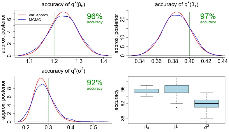
Figure 1: Upper panels and lower left panel: approximate posterior density functions forβ0,
β1andσ2based on the variational approximation scheme described by Algorithm 1 and MCMC, for the first replication of the simulation study described in the text. Accuracy values, according to (11), with the exact posterior density function replaced by the MCMC-based posterior density function are also given. Lower right panel: Side-by-side boxplots of all 1000 accuracy values obtained for each parameter in the simulation study.
logp(y;q) = 12(K+p) + log Γ(12(K+ 1))−log(π)−log(A)−1T log(y!)−12plog(σβ2) +yTCµq(β,u)−1T expnCµq(β,u)+12diagonal(CΣq(β,u)CT)o
− 1
2σ2
β
{kµq(β)k2+ tr(Σ
q(β))}+12log|Σq(β,u)|
−12(K+ 1) log12{kµq(u)k2+ tr(Σq(u))}+µq(1/a) −log(µq(1/σ2)+A−2) +µq(1/σ2)µq(1/a).
Initialize: µq(1/σ2) > 0, µq(β,u) a (p+K)×1 vector and Σq(β,u) a (p+K)×(p+K) positive definite matrix.
Cycle:
wq(β,u)←expnCµq(β,u)+ 12diagonal(CΣq(β,u)CT)o
Σq(β,u)←
CTdiag{wq(β,u)}C+
σβ−2Ip 0
0 µq(1/σ2)IK
−1
µq(β,u)←µq(β,u)+Σq(β,u)
CT(y−wq(β,u))−
σβ−2Ip 0
0 µq(1/σ2)IK
µq(β,u)
µq(1/σ2)←
K+ 1
2µq(1/a)+kµq(u)k2+ tr(Σ
q(u))
; µq(1/a)←1/(µq(1/σ2)+A−2).
until the absolute change in p(y;q) is negligible.
Algorithm 1: Iterative scheme for determination of the optimal parameters in q∗(β,u),
q∗(σ2) and q∗(a) for the posterior density function approximation (9).
I replicated 1000 data-sets corresponding to the simulation setting
yij|Ui ∼Poisson (exp(β0+β1xij+Ui)), Ui|σ2∼N(0, σ2),
1≤i≤m, 1≤j≤n,
σ2|a∼Inverse-Gamma(12,1/a), a∼Inverse-Gamma(12, A−2), β∼N(0, σ2βI)
(10)
The hyperparameters were set atσβ =A= 105and the sample sizes werem= 100,n= 10.
Note that (10) is a special case of (8) withZ=Im⊗1n, where1n is then×1 vector with
all entries equal to one.
For each data-set I obtained approximate posterior density functions for β0,β1 and σ2 using both Algorithm 1 and Markov chain Monte Carlo (MCMC). For MCMC I used the package BRugs (Ligges et al., 2012) within the Rcomputing environment (R Development Core Team, 2013) with a burnin of size 5000 followed by the generation of 5000 samples, with a thinning factor of 5. This resulted in MCMC samples of size 1000 being retained for inference. The iterations in Algorithm 1 were terminated when the relative change in logp(y;q) fell below 10−4.
Figure 1 displays side-by-side boxplots of accuracy scores defined by
accuracy(q∗) = 100
1−12
Z ∞
−∞
q∗(θ)−p(θ|y) dθ
%. (11)
Figure 1 allows visual assessment of the variational approximate posterior density func-tions against the MCMC-based benchmark for a single replication of the simulation study. The accuracy is seen to be excellent forβ0 and β1 and very good for σ2.
As discussed in Knowles and Minka (2011), convergence of non-conjugate variational message passing is not guaranteed. In the simulation study the algorithm converged in all replications regardless of starting values, but in about 2% of the cases this required some adjustment to avoid inverting a singular matrix in the Σq(β,u) update during the early iterations. The adjustment involves addingεI to the matrix requiring inversion, withε >0 chosen so that the condition number stayed below 1016. In almost all cases, this adjustment was only necessary for the first few iterations.
In this section we have shown that non-conjugate variational message passing leads to an attractive variational inference algorithm for Poisson mixed models. Since the exponential moments of Multivariate Normal random vectors are available in closed form, no quadrature is required in the Poisson case. Other generalized linear mixed models, such as logistic mixed models, require quadrature. The logistic analogue of (8) is such that only univariate quadrature is required. Details are given in Appendix B of Tan and Nott (2013).
5.2 Heteroscedastic Additive Model
This illustration involves analysis of data from the Californian air pollution study described in Breiman and Friedman (1985). The response variable is
y= ozone concentration (ppm) at Sandburg Air Force Base
and three predictors variables are
x1 = pressure gradient (mm Hg) from Los Angeles International Airport to Daggett, California,
x2 = inversion base height (feet)
and x3 = inversion base temperature (degrees Fahrenheit).
The data comprises 345 measurements on each of these 4 variables. Let (xi1, xi3, xi3, yi),
1≤i≤345 denote the full regression data set. We entertained the heteroscedastic additive model
yi∼N
β0+f1(x1i) +f2(x2i) +f3(x3i),exp γ0+h1(x1i) +h2(x2i) +h3(x3i)
, (12)
for 1≤i≤345. Herefj and gj,j = 1,2,3, and smooth but otherwise arbitrary functions.
Bayesian mixed model-based penalized splines (e.g. Ruppert et al., 2003) were used to model the smooth functions as follows:
fj(x) = βjx+ Kj
X
k=1
ujkzjk(x), ujk iidN(0, σuj2 )
and hj(x) = γjx+ Kj
X
k=1
vjkzjk(x), vjk iid N(0, σvj2 ).
0 1000 2000 3000 4000 5000
0
5
10
15
20
25
30
contribution to mean
inversion base height var. approx.
MCMC
−50 0 50 100
0
5
10
15
20
25
30
contribution to mean
Daggett pressure gradient
30 40 50 60 70 80 90
0
5
10
15
20
25
30
contribution to mean
inversion base temperature
0 1000 2000 3000 4000 5000
0
5
10
15
contribution to standard deviation
inversion base height
−50 0 50 100
0
5
10
15
contribution to standard deviation
Daggett pressure gradient
30 40 50 60 70 80 90
0
5
10
15
contribution to standard deviation
inversion base temperature
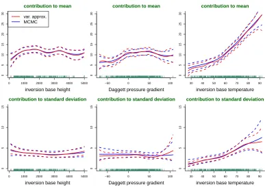
Figure 2: Upper panels: approximate pointwise posterior means and 95% credible sets for the mean function contributions f1, f2 and f3 according to the heteroscedastic additive model (12). Vertical alignment of the estimated functions is described in the text. Lower panels: approximate pointwise posterior means and 95% cred-ible sets for the standard deviation function contributions exp(h2/2), exp(h2/2) and exp(h3/2). Approximate Bayesian inference is based on both non-conjugate variational message passing and MCMC.
where iid stands for ‘independently and identically distributed as’. The{zjk : 1≤k≤Kj},
j = 1,2,3, are spline bases of sizes Kj respectively. My default for the zjk are suitably
transformed cubic O’Sullivan splines, as described in Section 4 of Wand and Ormerod (2008). The priors on the regression coefficients and standard deviation parameters are
βj iidN(0, σβ2), γj iidN(0, σγ2), σuj iid Half-Cauchy(Au), σvj iid Half-Cauchy(Av). (14)
The regression data replaced by standardized versions and the hyperparameters were set to be σβ = σγ = Au = Av = 105, corresponding to non-informativity. The results were
transformed to the original units after fitting. The basis function sizes were all fixed at
K1 =K2=K3= 18.
The Bayesian model given by (12), (13) and (14) admits a closed form non-conjugate variational message passing algorithm, with the regression coefficients for the full mean and variance functions each being Multivariate Normal. Details are given in Menictas and Wand (2014). Figure 2 shows the estimated mean function (fj) contributions, and the
and MCMC. The MCMC inference was carried out in the same fashion as for the illustra-tion described in Secillustra-tion 5.1. The abbreviated names inversion base height, Daggett pressure gradient and inversion base temperature are used for x1, x2 and x3. The estimatedf1 display is vertically aligned to match the response data by evaluating the esti-mate off2 atx2 and estimate off3 atx3, wherex2 and x3 are the sample means of thex2i
and x3i, respectively. Analogous alignment strategies were used for thef2 and f3 displays. Figure 2 shows that there is excellent agreement between non-conjugate variational message passing, with Multivariate Normal coefficient vectors, and MCMC. The former approach is considerably faster. The heteroscedasticity is seen to be relatively mild for inversion base heightandDaggett pressure gradient. However, there is pronounced heteroscedasticity ininversion base temperature that is captured by model (12).
Acknowledgments
This research was partially supported by Australian Research Council Discovery Project DP110100061. The author is grateful to Cathy Lee, Jan Luts, Marianne Menictas, Tom Minka, David Nott and Linda Tan for their comments.
Appendix A: Proof of Theorem 1
Proof of (a)
For the upper-left block of U note that µ = Ση1 and so dη1µ = Σdη1. Theorem 6 of Magnus and Neudecker (1999) leads toDη1µ=Σ. The lower-right block ofU involves the relationΣ=−1
2{vec
−1(D+T
d η2)}−1 given in (5). Then Rule 3.3.5 in Wand (2002) and the identity
vec(ABC) = (CT ⊗A) vec(B) (15)
leads to
dη2vec(Σ) = 2 vec(Σ{vec−1(D+dTdη2)}Σ) = 2(Σ⊗Σ)D+dT dη2. Hence, making use of Theorem 13 (b), Chapter 3, of Magnus and Neudecker (1999),
Dη2vec(Σ) = 2(Σ⊗Σ)D
+T
d = 2DdD
+
d(Σ⊗Σ)D
+T
d =DdS = (SD
T d)T.
The expression for the lower-left block of U follows from
dη2µ= 2Σ{vec
−1(D+T
d dη2)}Ση1 = 2 vec(Σ{vec
−1(D+T
d dη2)}µ) = 2(µT ⊗Σ)D+dT dη2 where Rule 3.3.5 in Wand (2002) and (15) have been used again. This gives
Dη2µ= 2(µ
T ⊗Σ)D+T
d ={2D
+
d(µ⊗Σ)}
T ={2D+
d(µ⊗Id)(1⊗Σ)}
T = (MΣ)T.
For the upper-left block note that, from (5),dη1vec(Σ) =0dη1 and so Dη1vec(Σ) =0.
Proof of (b)
Proof of (c)
The upper-left block is var(x) =Σ. The lower-right block is
var{vech(xxT)} = D+d var{vec(x1xT)}D+dT =D+d var(vec(x⊗xT))D+dT
= D+d (Id2+Kd)(Σ⊗Σ+Σ⊗µµT +µµT ⊗Σ)D+dT
where (15) and Theorem 4.3 (iv) of Magnus and Neudecker (1979) has been used. Here
Kd denotes thecommutation matrix of orderd, defined byKd(A⊗B) = (B⊗A)Kdfor
arbitrary d×d matrices A and B. Noting the identity 12Dd+(Id2 +Kd) =D+d, which is an immediate consequence of (15) in Chapter 3 of Magnus and Neudecker (1999), one then gets
var{vech(xxT)}=S+ 2D+d(Σ⊗µµT +µµT ⊗Σ)D+dT.
Theorem 12(a), Chapter 3, of Magnus and Neudecker (1999) states that KdDd = Dd,
which implies that
D+d ={(KdDd)TKdDd}−1DTdKTd = (DTdKTdKdDd)−1DTdKd=D+dKd. (16)
Here I have usedKT =K−d1 =Kdas stated in (2) of Chapter 3 of Magnus and Neudecker
(1999). The identityD+d =D+dKd leads to
D+d(Σ⊗µµT)Dd+T=D+dKd(Σ⊗µµT)D+dT=D+d(µµT⊗Σ)KTdD+dT=D
+
d(µµ
T⊗Σ)D+T d
leading to var{vech(xxT)}=S+ 4Dd+(µµT ⊗Σ)D+dT. Since
(µµT ⊗Σ) = (µ⊗Σ)(µT ⊗Id) = (µ⊗Id)(1⊗Σ)(µT ⊗Id) = (µ⊗Id)Σ(µ⊗Id)T.
I conclude that
var{vech(xxT)}=S+MΣMT.
The (i, j) entry of the lower-left block is
cov(vech(xxT)i, xj) = cov({D+dvec(xx T)}
i, xj) = d2 X
k=1
(D+d)ikcov(vec(xxT)k, xj). (17)
Letbxcdenote the largest integer less than or equal tox. Then using one of the fundamental identities for generalized cumulants given on page 58 of McCullagh (1987),
cov(vec(xxT)k, xj) = cov(xk−db(k−1)/dcxb(k−1)/dc+1, xj)
= µk−db(k−1)/dcΣb(k−1)/dc+1,j+µb(k−1)/dc+1Σk−db(k−1)/dc,j
= (Σ⊗µ)kj+ (µ⊗Σ)kj.
Combining this with (17), the lower-left block equals D+d(Σ⊗µ+µ⊗Σ). But, courtesy of (16), this equals
Proof of (d)
It is straightforward to verify that
Σ ΣMT
MΣ S+MΣMT
Σ−1+MTS−1M −MTS−1
−S−1M S−1
=Id+d(d+1)/2. The stated expression for V−1 immediately follows.
Proof of (e)
V−1U =
Σ−1+MTS−1M −MTS−1
−S−1M S−1
Σ 0
MΣ SDTd
=
I −MTDTd
0 DTd
.
Proof of (f )
First note that
V−1U
g
vec(G)
=
I −MTDTd
0 DTd
g
vec(G)
=
g−MTDTd vec(G)
DTdvec(G)
.
With the help of Lemma 1 and (15) one then has
MTDTd vec(G) = 2(µT ⊗Id)D+dTD T
dvec(G) = 2(µT ⊗Id) vec(G) = 2Gµ
and the stated result is obtained.
Appendix B: Proof of Theorem 2
Proof of (a)
Let Aij and Bij, respectively, denote the (i, j) entry of A and B. Then a listing of the
entries ofQ(A) reveals that its entry is (i, j) is
Q(A)ij =Ai,b(j−1)/dc+1Ai,j−db(j−1)/dc, 1≤i≤n, 1≤j≤d2. (18)
Similarly, theith entry of vec(B) is
vec(B)j =Bj−db(j−1)/dc,b(j−1)/dc+1, 1≤j≤d2. (19) Hence
{Q(A) vec(B)}i = d2
X
j=1
Ai,b(j−1)/dc+1Ai,j−db(j−1)/dcBj−db(j−1)/dc,b(j−1)/dc+1
= d X j=1 + 2d X
j=d+1
+. . .+
d2 X
j=(d−1)d+1
Ai,b(j−1)/dc+1Ai,j−db(j−1)/dc ×Bj−db(j−1)/dc,b(j−1)/dc+1
=
d X
j=1
Ai1AijB1j+ d X
j=1
Ai2AijB2j+. . .+ d X
j=1
AidAijBdj
= d X j=1 d X
j0=1
and the result follows immediately.
Proof of (b)
Lettingbi denote the ith entry ofband making use of (18) one has
{Q(A)Tb}j =
n X
i=1
{Q(A)T}jibi= n X
i=1
Q(A)ijbi
=
n X
i=1
biAi,b(j−1)/dc+1Ai,j−db(j−1)/dc.
Application of (19) to ATdiag(b)A gives
vec(ATdiag(b)A)j = (ATdiag(b)A)j−db(j−1)/dc,b(j−1)/dc+1 =
n X
i=1
bi(AT)j−db(j−1)/dc,iAi,b(j−1)/dc+1
=
n X
i=1
biAi,b(j−1)/dc+1Ai,j−db(j−1)/dc={Q(A)Tb}j
which proves equality between Q(A)T band vec(ATdiag(b)A).
Appendix C: Derivation of Algorithm 1
Derivation of q∗(σ2)
logq∗(σ2) = Eq{logp(σ2|rest)}+ const
= {−12(K+ 1)−1}log(σ2)− {12Eqkuk2+µq(1/a)}/σ2+ const. where ‘const’ denotes terms not involvingσ2. Using
Eqkuk2 =kµq(u)k2+ tr(Σq(µ)) I then get q∗(σ2)∼Inverse-Gamma(21(K+ 1), Bq(σ2)) where
Bq(σ2)= 1
2{kµq(u)k2+ tr(Σq(µ))}+µq(1/a).
Derivation of q∗(a)
logq∗(a) = Eq{logp(a|rest)}+ const
= (−1−1) log(a)−(µq(1/σ2)+A−2)/a+ const. This givesq∗(a)∼Inverse-Gamma(1, Bq(a)) where
Derivation of the (µq(β,u),Σq(β,u)) Updates
Note that
Eq{logp(y,β,u, σ2, a)} = Eq{log p(y|β,u) + log p(β,u|σ2) + log p(σ2|a) + logp(a)}
= S+ terms not involvingµq(β,u) orΣq(β,u)
where
S ≡S(µq(β,u),Σq(β,u))≡Eq{logp(y|β,u) + log p(β,u|σ2)}.
Then
S = yTCµq(β,u)−1T expnCµq(β,u)+12diagonal(CΣq(β,u)CT)o
−1 2tr
σβ−2Ip 0
0 µq(1/σ2)IK
{µq(β,u)µTq(β,u)+Σq(β,u)}
−12(p+K) log(2π)−12plog(σβ2)−12K Eq{log(σ2)} −1T log(y!)
and so
dµq(β,u)S = y
TCdµ q(β,u)
−1Tdiag[exp{Cµq(β,u)+12diagonal(CΣq(β,u)CT)}]Cdµq(β,u)
−µTq(β,u)
σβ−2Ip 0
0 µq(1/σ2)IK
dµq(β,u)
= hy−exp{Cµq(β,u)+12diagonal(CΣq(β,u)CT)}
iT C
−µTq(β,u)
σβ−2Ip 0
0 µq(1/σ2)IK
dµq(β,u).
Thus, by Theorem 6, Chapter 5, of Magnus and Neudecker (1999),
{Dµq(β,u)S}
T = CT hy−exp{Cµ
q(β,u)+12diagonal(CΣq(β,u)C
T)}i
−
σβ−2Ip 0
0 µq(1/σ2)IK
µq(β,u).
Next, using Theorem 2 of Section 4 and Rule 3.3.2 of Wand (2002),
dvec(Σ
q(β,u))S = −1
Tdiag[exp{Cµ
q(β,u)+ 12diagonal(CΣq(β,u)CT)}]12Q(C)dvec(Σq(β,u))
−12vec
σ−β2Ip 0
0 µq(1/σ2)IK
T
dvec(Σq(β,u)) =
−12exp{Cµq(β,u)+12diagonal(CΣq(β,u)CT)}TQ(C)
−1 2vec
σ−β2Ip 0
0 µq(1/σ2)IK
T
dvec(Σq(β,u)
= −12vec
CTdiag[exp{Cµq(β,u)+12diagonal(CΣq(β,u)CT)}]C +
σ−β2Ip 0
0 µq(1/σ2)IK
T
and so
vec−1
(Dvec(Σq(β,u))S)
T = −1
2 C
Tdiag[ exp{Cµ
q(β,u)+ 12diagonal(CΣq(β,u)CT)}]C
+
σ−β2Ip 0
0 µq(1/σ2)IK
!
.
References
M. Braun and J. McAuliffe. Variational inference for large-scale models of discrete choice. Journal of the American Statistical Association, 105:324–335, 2010.
L. Breiman and J. Friedman. Estimating optimal transformations for multiple regression and correlation (with discussion). Journal of the American Statistical Association, 80: 580–619, 1985.
J. Hensman, M. Rattray, and N. D. Lawrence. Fast variational inference in the conjugate exponential family. In P. Bartlett, F.C.N. Pereira, C.J.C. Burges, L. Bottou, and K.Q. Weinberger, editors,Advances in Neural Information Processing Systems 25, pages 2897– 2905, 2012.
D. A. Knowles and T. P. Minka. Non-conjugate message passing for multinomial and binary regression. In J. Shawe-Taylor, R.S. Zamel, P. Bartlett, F. Pereira, and K.Q. Weinberger, editors, Advances in Neural Information Processing Systems 24, pages 1701–1709, 2011. U. Ligges, S. Sturtz, A. Gelman, G. Gorjanc, and C. Jackson. BRugs. Fully-interactive R interface to the OpenBUGS software for Bayesian analysis using MCMC sampling, 2012. URLhttp://cran.r-project.org. R package version 0.8-0.
J. R. Magnus and H. Neudecker. Matrix Differential Calculus with Applications in Statistics and Econometrics, Revised Edition. Wiley, Chichester UK, 1999.
J.R. Magnus and H. Neudecker. The commutation matrix: some properties and applica-tions. The Annals of Statistics, 7:381–394, 1979.
P. McCullagh. Tensor Methods in Statistics. Chapman and Hall, London, 1987.
M. Menictas and M. P. Wand. Variational inference for heteroscedastic semiparametric regression. 2014. Unpublished manuscript.
T. Minka and J. Winn. Gates: A graphical notation for mixture models. Microsoft Research Technical Report Series, MSR-TR-2008-185:1–16, 2008.
T. Minka, J. Winn, J. Guiver, and D. Knowles. Infer.NET 2.5, 2013. URL http:// research.microsoft.com/infernet. Microsoft Research Cambridge.
R Development Core Team. R: A Language and Environment for Statistical Comput-ing. R Foundation for Statistical Computing, Vienna, Austria, 2013. URL http: //www.R-project.org/. ISBN 3-900051-07-0.
D. Ruppert, M. P. Wand, and R. J. Carroll. Semiparametric Regression. Cambridge Uni-versity Press, New York, 2003.
L. S. L. Tan and D. J. Nott. Variational inference for generalized linear mixed models using partially noncentered parametrizations. Statistical Science, 28:168–188, 2013.
M. J. Wainwright and M. I. Jordan. Graphical models, exponential families, and variational inference. Foundation and Trends in Machine Learning, 1:1–305, 2008.
M. P. Wand. Vector differential calculus in statistics. The American Statistician, 56:55–62, 2002.
M. P. Wand and J. T. Ormerod. On semiparametric regression with O’Sullivan penalized splines. Australian and New Zealand Journal of Statistics, 50:179–198, 2008.
M. P. Wand, J. T. Ormerod, S. A. Padoan, and R. Fr¨uhwirth. Mean field variational Bayes for elaborate distributions. Bayesian Analysis, 6(4):847–900, 2011.