A New Method for the Analysis of Misaligned Journal Bearing

Tribology in Industry

www.tribology.rs

A New Method for the Analysis of Misaligned

Journal Bearing

H.U. Jamali

a

_{, A. Al-Hamood}

a

a_{University of Kerbala, Kerbala, Iraq.}

Keywords: 3D Misalignment Finite length Numerical solution Boundary conditions Load convergence

A B S T R A C T

One of the most problems that affects the performance of the journal bearing is the shaft misalignment. Misalignment may result due to installation error, shaft deformation, manufacturing error, bearing wear, etc. This paper presents a solution for the misaligned journal bearing problem under hydrodynamic regime. The Reynolds equation has been solved numerically for a finite length bearing based on the finite difference method. The solution demonstrates a new model for the representation of the 3D misalignment geometry and also a detailed procedure for the implementation of the boundary condition in the numerical solution is explained. Furthermore, the convergence of the solution to the required load is investigated. The results reveal a severe thinning in the levels of film thickness and significant rising of the maximum pressure value when the misalignment is taken into consideration.

© 2018 Published by Faculty of Engineering Corresponding author:

Hazim U. Jamali University of Kerbala, Kerbala, Iraq.

E-mail: [email protected]

1. INTRODUCTION

The contact problem in the case of journal bearing is solved in general under the consideration of hydrodynamic regime of lubrication. In this regime, the surfaces of contact are separated by a relatively thick film of lubricant (in the order of microns) as compared with the elastohydrodynamic lubrication (a fraction of micron). The most typical example for hydrodynamic lubrication is the journal bearing and for the elastohydrodynamic lubrication are gears and ball bearings. The journal bearing consists of shaft (journal) carrying the load which rotates inside the bearings under conformal contact. The clearance between the journal and the bearing (difference between

their radii) is relatively small which is in most typical applications in the order of tens of microns. In the case of ideal operation of the journal bearing system, the shaft longitudinal axis and the line between the bearing centers are parallel. The deviation from this parallelism could cause negative consequences on the performance of the bearing. Due to the small clearance between the surfaces, a certain little deviation may result in a direct contact. Such deviation may result from the deflection of the shaft under load, mounting errors, manufacture errors, etc. The system is called an aligned journal bearing in the former case and misaligned journal bearing in the later. The problem of hydrodynamic lubrication of both aligned and misaligned journal bearings has

R

ES

EA

R

drawn the attention of researchers from decades. This can be attributed to the wide range of journal bearing use in industrial applications. Typical applications include IC engine, compressors, turbines, etc.

Mokhtar et al. [1] solved the problem of misalignment for a length to diameter ratio

(𝐿/𝐷) of unity. Their results revealed that the thermal effects are more obvious when the misalignment is taking into consideration. Safar et al. [2] considered turbulent regime in the analyses of misaligned journal bearing. The result showed that the present of misalignment increases the power consumption in comparison with aligned bearing. Sun et al. [3] studied experimentally the effect of misalignment due to shaft bending. The results showed an obvious effect on the pressure distribution and the film thickness levels. Nikolakopoulos and Papadopoulos [4] presented a model which described the relation between the misalignment and the wear as well as the friction force. Jang and Khonsari [5] analyzed the misaligned journal bearing based on a 3D mass-conservative model. The numerical results showed how the misalignment affects the system performance. Zhen-peng et al. [6] studied the effect of shaft misalignment due to asymmetric rotor structure on the performance of journal bearing system. They used a new model to represent the misalignment based on stepped shaft in a rotor bearing system. Qiang et al. [7] studied the effect of misalignment using computational fluid dynamics where a new approach was used for mesh moving during the simulation of the fluid dynamics. Xu et al. [8] also investigated the effect of turbulent and thermohydrodynamic on the static and dynamic characteristic of journal bearing with the consideration of misalignment. The turbulent and thermal effect in combination with the misalignment was found to have considerable effect on the system performance. Rajput and Sharma [9] investigated the journal misalignment together with different forms of geometric imperfection on the characteristics of hybrid system of journal bearing. The numerical results illustrated the significant deteriorated of the performance of the system due to the combination of misalignment and geometric imperfection. Fangrui et al. [10] analyzed the journal bearing problem considering vertical misalignment only. Jao et al. [11] used finite

element method to investigate the misaligned journal bearing where the anisotropic slip is considered in the analysis. Zernin et al. [12] studied many factors related to the deviation in bearing shape including the misalignment of the shaft. Rajput et al. [13] examined the effect of geometric irregularities of a journal bearing system where the shaft misalignment is taking into consideration.

Although extensive work has been carried out on the lubrication analyses of journal bearing, there is a few details in the literature about the following subjects: (1) comprehensive and detailed mathematical modeling of the geometry of misaligned journal bearing, (2) the way in which the boundary conditions is implemented in the numerical solution and (3) how the convergence to the applied load is obtained. In this paper all these issues are considered in details where a full numerical solution (using finite difference method) for a finite length journal bearing is presented. The effects of misalignment in the horizontal and vertical planes are considered where the solution is based on the use of Reynolds boundary conditions method. A detailed procedure for the solution using this method is specified. The misalignment effects on the geometry of the system are presented in a relatively simple and efficient model together with a route for the convergence criteria of the load.

2. GOVERNING EQUATIONS

The governing equations for isothermal hydrodynamic problem of journal bearing are Reynolds equation and the film thickness equation. The well-known Reynolds equation is [14]:

0 12

12

3 3

        

  

  

      

  

  



x h u z p h z x p h

x   m (1)

m

u is the mean entrainment velocity of the two surfaces which is given by:

2

b j m

u u

u  

Since the surface velocity of the bearing (u_b) is zero,

x



R



and

u

_j



R



[15], the Reynolds equation for this hydrodynamic problem is

0 6

6

3 3

2  

      

  

  

      

  

  



  

  

h z

p h z p h

R (2)

The film thickness equation around the journal is [16]:

)) cos( 1

( 









c _r

h (3)

3. GEOMETRY OF THE JOURNAL BEARING

Figure 1 shows a schematic representation for an aligned journal- bearing system. Figure 1a illustrates a 3D drawing and Fig. 1b shows a side view for the system where the journal (shaft) in its equilibrium position.

Fig. 1. Schematic drawing of the journal-bearing. (a) 3D representation; (b) side view.

It can be seen in Fig. 1b that the journal centre,

𝑂_𝑗shifted from the bearing centre, 𝑂_𝑏 by the eccentricity distance 𝑒. The three point 𝑂₁, 𝑂₃

and 𝑂₂represent the centre of the journal at the right, middle and left side of the bearing. For the case of aligned bearing (which is shown in this figure), these three points lie on horizontal line. In the side view, these points coincide with each other and appear as one point which is denoted by 𝑂_𝑗 in Fig. 1b. The case of misaligned journal bearing will be discussed later. In figure (1-b) the coordinate system is fixed at the bearing centre 𝑂_𝑏. The line between 𝑂_𝑗and 𝑂_𝑏 inclines to the 𝑦 axis by angle 𝛽 which is called the attitude angle. The angle 𝜃, measured from the 𝑦 axis, will be used as angular coordinate for the points around the journal surface.

3.1 Geometry of the misaligned journal bearing

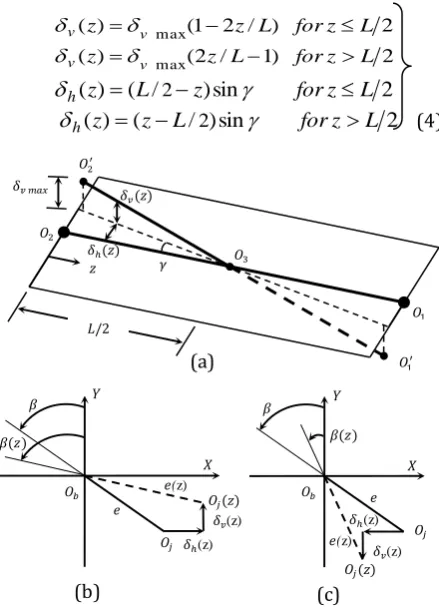
For the case of misaligned journal bearing, the line of centres 𝑂1𝑂2 that shown in Fig. 1a is deviated from the horizontal line as shown in

Fig. 2a. This deviation may occur in the vertical plane, horizontal plane or both planes where the later represents a 3D misalignment problem. The 3D misalignment case is shown in this figure where the new position of the line 𝑂₁𝑂₂ is illustrated through drawing the line 𝑂1′𝑂2′. The vertical and horizontal deviations are defined by

𝛿𝑣and 𝛿ℎ respectively. Both deviations vary linearly from a maximum value at the edges to zero at the centre of the middle section of the journal, 𝑂₃. Therefore, 𝛿_𝑣and 𝛿_ℎ are functions of

𝑧 axis which is measured from the left side of the horizontal plane that shown in Fig. 2a. The deviation at the edges, 𝛿𝑣 𝑚𝑎𝑥 in the vertical plane and the angle of deviation, 𝛾 in the horizontal plane are chosen as input parameters to investigate the effect of misalignment on the performance of the system. It is worth mentioning that for the case when 𝛾 = 0, a pure vertical misalignment is considered and in the same way only horizontal misalignment is a result of the case when 𝛿_{𝑣 𝑚𝑎𝑥}= 0. The vertical and horizontal deviation at any 𝑧 position can be calculated in terms of 𝛿_{𝑣 𝑚𝑎𝑥} and 𝛾 respectively as (see Fig. 2a).

2 )

/ 2 1 ( )

(z _{v max} z L forz L

v   



2 )

1 / 2 ( )

(z _{v max} z L forz L

v   



2 sin

) / ( )

(z L 2 z forz L

h    



_h(z)(zL/2)sin forzL 2 (4)

Fig.2. Geometry of the misaligned journal bearing system. (a) 3D representation for the deviation of the journal axis; (b) Deviation of the journal centre

(𝑧 ≤ 𝐿/2); (c) Deviation of the journal centre

(𝑧 > 𝐿/2).

(a) (b)

𝑂1

𝑂2

𝑂3

𝐿

𝑌

𝛽

𝑒 𝑂𝑏

𝑂𝑗

𝜃

𝑋

𝜃 − 𝛽

𝑧 𝑂3

𝑂1

𝑂2

𝛿𝑣 𝑚𝑎𝑥 _𝛿 𝑣(𝑧)

𝛿ℎ(𝑧)

𝛾

𝐿/2 𝑂2′

𝑂1′

(b) (c)

𝑋 𝑌

𝛽

𝛽(𝑧)

𝑒

𝛿ℎ(z) 𝛿𝑣(z) 𝑒(z)

𝑂𝑏 _𝑂

𝑗(𝑧)

𝑂𝑗

𝑋 𝑌

𝛽

𝛽(𝑧)

𝑒 𝛿ℎ(z)

𝛿𝑣(z) 𝑒(z) 𝑂𝑏

𝑂𝑗(𝑧)

The centre of any circle of the shaft along the length of the bearing lies on the horizontal line

𝑂₁𝑂₂ for the aligned bearing and shifted from the corresponding bearing centre by a constant distance 𝑒 as discussed previously. This means in other wards that 𝑒 and 𝛽 are not function of 𝑧. The case is entirely different when the misalignment is taken into consideration. Figure 2b illustrate a section for the journal and the bearing at any distance when 𝑧 ≤ 𝐿/2 for misaligned journal. The centre of the journal shifts from its original position 𝑂_𝑗 to 𝑂_𝑗′ _{due to}

the horizontal misalignment 𝛿_ℎ(𝑧) and the vertical misalignment 𝛿𝑣(𝑧) at this section. This new position of the journal centre at this section consequently results in a new eccentricity and attitude angle. Therefore, the eccentricity and the attitude angle both depend on 𝑧 position of the section under consideration. These new 𝑒(𝑧)

and 𝛽(𝑧) need to be determine a long the whole length of the bearing in order to calculate the gap between the journal and the bearing. The calculation of this gap represents an essential step in the solution of Reynolds equation. These can be easily determined in terms of 𝑒 and 𝛽

from the trigonometric relations for 𝑧 ≤ 𝐿/2:

2 2 )) ( sin ( )) ( cos ( )

(z e z e z

e  _v  _h (5)

and ) ( cos ) ( sin tan ) ( z e z e Arc z v h         (6)

Similarly, the corresponding equation for any section at 𝑧 > 𝐿/2 that shown in Fig. 2c can be given by: 2 2 )) ( sin ( )) ( cos ( )

(z e z e z

e  _v  _h (7)

and ) ( cos ) ( sin tan ) ( z e z e Arc z v h         (8)

where _h(z), _v(z)are given by eq. 4.

Therefore, the film thickness equation (eq. 3) can be written for the case of misaligned journal bearing in terms of 𝑒(𝑧) and 𝛽(𝑧) in the following form: ))) ( cos( ) ( 1 ( ) ,

( z C z z

h



 



_r







₍₉₎ where C z e z r ) ( ) (  

4. NUMERICAL SOLUTION

In the case of journal bearing, Reynolds equation can be solved analytically only for particular cases. This includes the well known assumption of short bearing and long bearing solutions [17]. In the former case the pressure gradient in the 𝑥

direction (p x) is ignored while in the later case, the pressure gradient in the 𝑧 direction (

z p 

 ) is neglected. This assumption is based on the length to diameter ratio (𝐿/𝐷). According to this solution, the bearing is considered short when 𝐿/𝐷 < 1 and long when 𝐿/𝐷 > 2. Consequently, for the finite length bearing (1 < 𝐿/𝐷 < 2), a numerical solution for Reynolds equation is required. In this paper finite difference method is used for the solution of hydrodynamic problem of finite length journal bearing. This solution is achieved by dividing the solution plane (plane (,z)) to 𝑛 ∗ 𝑚 mesh

points in the circumferential and longitudinal direction of the bearing respectively. Figure 3 shows point (𝑖, 𝑗) in this solution domain which is surrounded by the four neighbour mesh points. The pressure gradient in the circumferential direction can be discretized using central difference as following:

Fig. 3. Part of the solution domain.                          

 II I

p h p h

p

h 6 6

6 3 3 3 (10) where

  



      

p p i j pi j

I , 1 , (10a)



  

      

p p i j pi j

II

, ,

1

(10b)

And the film thickness at the boundary of the control volume is taken as average value as:

∆𝑧/2

∆𝜃/2 (𝑖, 𝑗)

(𝑖 − 1, 𝑗) (𝑖 + 1, 𝑗)

(𝑖, 𝑗 − 1) (𝑖, 𝑗 + 1)

𝐼𝐼 𝐼

𝐼𝐼𝐼

  6 ) 2 / )) , ( ) , 1 ( (( 6 3

3 _{h i j h i j}

h

I

 

 (10c)

This equation represents the film thickness at point I and similar equations can also be written for the other points on the boundary of the control volume (points II, III and IIII).

Similarly, for the pressure gradient in the z direction: z z p h z p h z p h z IIII III j i                       6 6 6 3 3 ) , ( 3 (11)



  

z j i p j i p z p III     

 , 1 ,

(11-a)

  



z j i p j i p z p IIII     

 , , 1

(11-b)



 







       2 , 1 , 1 ) , ( j i h j i h h j i (12)

Substituting eqs. 10-12 into equation 2 and solving for the pressure at point 𝑖, 𝑗 yields,





                   ) , ( ) , ( ) , ( ) , ( ) , ( ) , ( 1 ) , ( 1 1 1 1 1 1 5 4 3 2 1 j i p a j i p a j i p a j i p a j i h j i h a a j i p o (13) where 4 3 2 1

0 b b b b

a    

2 2 z   







6 ) 2 / )) , ( ) , ( (( 3 1

1 j h i j

i h

b    ,

 6 ) 2 / )) ( ) , ( (( 3 2 , 1 j i h j i h

b   

 6 ) 2 / )) , ( ) , ( (( 3 3 1  

 h i j h i j

b ,  6 ) 2 / )) , ( ) , ( (( 3 4 1  

 h i j h i j

b

2

1







a ,a2 b2, a3 b1, a4b3, a5b4

The film thickness values that required in eqs. 10c and 12 are calculated using eq. 9.

Equation 12 is calculated at each point in the solution domain except the boundaries (i.e.

𝑛 − 1 ∗ 𝑚 − 1 points) where the pressure is zero. To carry out this calculation, an assumed pressure distribution is required over the solution domain which represents a first trial (𝑝_𝑜𝑙𝑑) in the iterative procedure. The new calculated pressure (𝑝_𝑛𝑒𝑤) values are then used as second trial which are substituted in the right hand side of eq (12). The process is continuing until the absolute difference between 𝑝_𝑛𝑒𝑤 and

𝑝𝑜𝑙𝑑 at each point is less than 1*10-7. In this paper the number of nodes in the numerical solution is 29241 nodes ( ∗ 𝑚 = 361 ∗ 81) This number is examined carefully where any increasing in the number of nodes beyond this limit has a trivial effect on the results. The examination is performed through comparing the maximum pressure and minimum film thickness for the cases when 𝑛 ∗ 𝑚 = 721 ∗ 161, 𝑛 ∗ 𝑚 = 361 ∗81,

𝑛 ∗ 𝑚 = 181 ∗ 41 and 𝑛 ∗ 𝑚 = 91 ∗ 21.

The bearing forces in 𝑋 and 𝑌 directions can be calculated by using the following equations:

  

I

L

X p z R d dz

F     0 0 sin ) , (    I L

Y p z R d dz

F    

0 0

cos ) ,

( (14)

when the convergence of the solution is achieved, the pressure values are available at all positions in the solution domain. Therefore, the forces in equations 14 can be easily calculated using numerical integration.

5. RESULTS

The model for the geometry of misalignment presented in this paper is compared with the work of Xu et al. [8] for the purpose of validation. They studied the effect of turbulent flow and thermohydrodynamic on the performance of misaligned journal bearing. In their paper the results for misaligned journal bearing without the consideration of turbulent and thermal effect were also presented. The following equation was used in their study for the calculation of film thickness where the derivation for this equation is not given in the paper.

) cos( ) 2 1 ( )

cos( _{o o}

o D z e e c

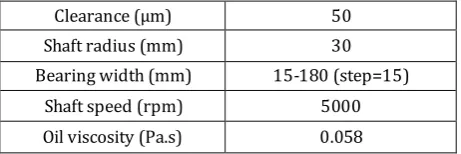
The results in the current work are based on the data for the journal bearing system that shown in table 1.

Table 1. Parameters of the journal-bearing.

Clearance (µm) 50

Shaft radius (mm) 30

Bearing width (mm) 15-180 (step=15)

Shaft speed (rpm) 5000

Oil viscosity (Pa.s) 0.058

Table 2 illustrates the values of minimum film thickness at different z-positions using the equation of reference [8] and the current model. It can be seen that the results are very close where the maximum error is 0.0154 % only. In the calculation of eq. (15) where the results are shown in this table, the following values are used for the purpose of comparison with the current work: e_o 27.372m, _48.984o

o

 ,

m 59.474 



e and 91.679o

where,

o

e

: eccentricity at

z



L

/

2

, _o: the attitude angle at

z



L

/

2

.

The other variables in this equation are rewritten in terms of _vmax and



in order to be consistence with the current work as:

2 2

max ( /2sin )

2  L 

e _v 

)) sin 2 / /( (

tan 2

/  1  _max 



  _o  _v L

Table 2. Minimum film thickness (µ𝑚) at different z-positions using the current model and equation of reference [8].

𝒛 = 𝟎 𝒛 = 𝟎. 𝟑𝑳 𝒛 = 𝟎. 𝟕𝑳 𝒛 = 𝑳

Equation of

Ref. [8] 8.5923 19.6173 20.7039 10.6004

Current

work 8.5910 19.6158 20.7037 10.5995

Error % 0.0154 0.007 0.001 0.008

In order to solve this hydrodynamic problem, the boundary conditions for Reynolds equation need to be known in advance along the boundaries of the solution plane in the axial and circumferential directions. Unfortunately this is not straightforwardly possible in the circumferential direction. In the axial direction, the boundary condition is zero pressure at the left and right hand sides of the bearing that

shown in Fig. 2a. This means in the numerical solution setting 𝑝 = 0 (ambient pressure) at all points around the journal when 𝑧 = 0 and 𝑧 = 𝐿. In the circumferential direction the position of boundary condition at the inlet lies at 𝜃 = 𝛽

where the gap between the journal and the bearing is maximum. However, the attitude angle is not known at this stage of the solution and its determination will be explained later. Several proposed methods where suggested for the determination of the position of the boundary conditions at the outlet where the pressure diminished. The solution of Reynolds equation results in positive pressure when

(𝜃 − 𝛽) < 180𝑜 _{and negative pressure when}

(𝜃 − 𝛽) > 180𝑜_{. This solution is well-known as} full Summerfield solution which is not possible practically as the fluid can not undertake negative pressure and cavitations occur to compensate the negative pressure. The pressure variation depends mainly on the shape (gap between the surfaces) of the film thickness. The gap between the shaft and the bearing decreases in the direction of shaft rotation towards a minimum value which leads to generate a positive pressure distribution due to the wedge effect. Afterward, as the film thickness increases in the divergence part, the assumption of continuous film lubrication predicts negative distribution for the pressure where larger amount of lubricant is pulled out in comparison with the amount flowed into the region. Another method to determine the outlet boundary condition is neglecting the negative pressure which leads to a pressure distribution ends at

(𝜃 − 𝛽) = 180𝑜_{. In this case the pressure drops} sharply to zero at (𝜃 − 𝛽) = 180𝑜 _{which is also} not the case in practice. The most widely used method in the solution of such contact problem is the Reynolds boundary conditions. This method ensures a gradual drop of pressure to zero at a position (𝜃 − 𝛽) > 180𝑜_{. This can be} achieved through setting 𝑝 = 0 and 𝜕𝑝 𝜕𝜃 = 0⁄

at (𝜃 − 𝛽)𝐼_{≤ (𝜃 − 𝛽) ≤ 360}𝑜_{. The position}

(𝜃 − 𝛽)𝐼 _{is determined through a number of} iterations [18]. The iterative procedure involves an assumption of (𝜃 − 𝛽)𝐼 _{which needs to be >>} 180. Starting from an angle close to the exit i.e.

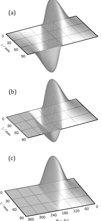
If there is any negative pressure is found, the assumed position of the boundary is updated to be (𝜃 − 𝛽)_𝑛𝑒𝑤𝐼 _{= (𝜃 − 𝛽)}𝐼_{− ∆𝜃}𝑜_{. The step ∆𝜃}𝑜 _is the mesh size in the circumferential direction. The iterations are continued until the pressure distribution is completely positive. Figure 4 shows some of the results during the iterative procedure where Fig. 4a shows the Full Summerfield solution as first iteration, Fig. 4b shows the results after a number of iteration where part of the pressure is still negative and Fig. 4c shows the result of the final iteration where the whole pressure distribution is positive.

Fig. 4. Pressure distribution throughout the solution of Reynolds boundary conditions method. (a): Full Summerfield solution as first iteration; (b): Result after number of iterations; (c): Final iteration. (The labels for the angle are not shown in Figs. a and b for clarity).

Figure 5 shows a sectional comparison for the pressure distribution at 𝑧 = 𝐿/2 during the iterative solution. Only 6 iterations are shown for the purpose of clarity. The red curve is for the case shown in Fig. 4a which consists of two

identical negative and positive halves. For this case, the change angle from positive to negative pressure is (𝜃 − 𝛽) = 180𝑜_{. The section for the} case shown in Fig. 4b is shown by the blue curve where part of the pressure distribution is still negative as explained previously. The corresponding final solution that shown in Fig. 4c is shown by the green curve where the pressure distribution is completely positive. The limit of pressure generation in this case extends beyond (𝜃 − 𝛽) = 180o_.

It is worth mentioning that the finding of the correct position of the boundary condition using Reynolds method is a relatively time consuming process. The time of solution is of great concern particularly in the case of misaligned journal bearing where another further iteration processes are required for the complete solution. However, this can be optimized by the best choice of the first assumed angular position in step 2 above. It can be seen in Fig. 5 that in the final iteration (curve number 3), the angular position of the boundary condition is at (𝜃 − 𝛽) = 204o_. Therefore, starting from (𝜃 − 𝛽) = 250o _{as a first} guess instead of (𝜃 − 𝛽) = 359o _{will saved} enormous number of iterations.

Fig.5. Sectional comparison at z = L/2 during the iterative solution of the Reynolds boundary condition method. (Red): Full Summerfield; (Blue) After number of iterations; (Green): Final iteration.

The attitude angle is required in order to calculate the film thickness equation as well as the geometry of the misaligned journal bearing. A relatively simple and efficient iterative procedure is used in this paper to calculate the attitude angle. This can be achieved by starting the solution with the assumption of zero attitude angle in equation 3. For the case when the load acts in the vertical direction (represents the most practical case in the applications of journal

z /_m m

0 30

60 90

no mis no crown pmax= 60.5 mpa mpa

z /_m m

0 30

60 90

after 100 iteration totaliteration 143

0 60 120 180 240 300 360

z / m_m

0 30

60 90

no mis no crown pmax= 60.5 mpa mpa

-60 -40 -20 0 20 40 60 80

0 60 120 180 240 300 360

P

/

Mpa

(θ-β)o

(a)

(b)

(c)

bearing), the force 𝐹_𝑌 in equation 8 represents the required load and 𝐹_𝑋 = 0 in this equation. After obtaining the convergence of the results, the attitude angle is increased (starting from zero) in an increment of 0.0001o _{and then}

equations 3 and 7 are recalculated. This routine is continuing until the force in the 𝑋-direction becomes zero (typically, less than 1E-5 N). The corresponding angle is the actual attitude angle.

Figure 6 shows the variation of the load with the change of the eccentricity ratio. The applied load in this case is 139.5 kN and the solution start with



_r 0.2 as first iteration. As the result

converged using this



_r, the pressure is integrated over the solution domain to obtain the load. The calculated load corresponding to

2 . 0

 r



is 20 kN which is much less the required value (139.5 kN). Therefore, the eccentricity ration increase in a coarse step as

r r

new

r  

  0.1 . When the calculated load

become close to the required load, the step decrease to be _rnew_r 0.001_r to avoid the oscillation of the results. If the calculated load become greater than the required load, the eccentricity ratio is reduced in a fine step (

r  001 .

0 ) until convergence is obtained.

Fig. 6. Load variation with the eccentricity ratio.

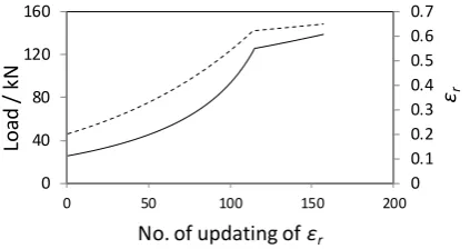
Figure 7 illustrates how the eccentricity ratio and the corresponding load change during the iteration. It requires 156 updating until convergence to the required load is obtained. The iteration starts with coarse step as explained above and then as the load becomes close to 0.9 of the required load, the steps changed to be fine. This can be seen clearly at iteration number 120. Afterward, the result converged smoothly to the required load. Without using a fine step, a fluctuation around the correct load is taking place as shown in Fig. 8 which shows the variation of the load during the iterative solution (updating of



r) in an enlarged scale for clarity. Although, the result

converged to 139.5 kN in this figure but in some cases the solution scheme becomes unstable and convergence cannot be obtained particularly in the misaligned journal. It is possible to avoid the coarse step in the first place but this approach requires enormous time for the solution.

Fig. 7. Changing of load (solid) and eccentricity ratio (dashed) throughout the iterations.

It is worth mentioning that each updating of the eccentricity ratio requires thousands of iteration to get the solution for Reynolds equation. The results shown in this figure, for example, requires 619889 iterations. The number of iteration, which is the title of the horizontal axis, shows only the number of eccentricity ratio updating for clarity.

Fig. 8. Fluctuating of the load throughout the iterations (enlarged scale).

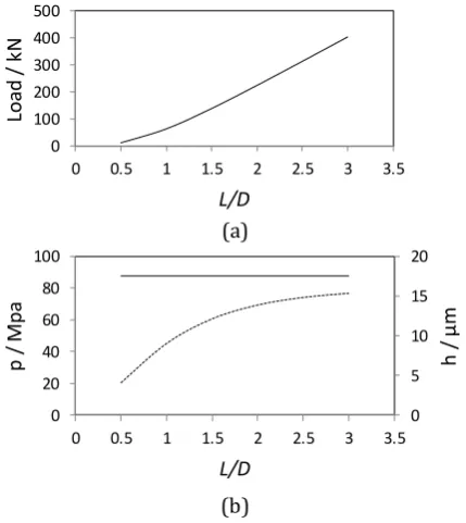
Figure 9 illustrates variation in the load, minimum film and maximum pressure using a wide range of 𝐿/𝐷 ratio based on a same value of 0.65 for the eccentricity ratio. The diameter is fixed in this figure to a value of 𝐷 = 60 mm. Figure (9-a) shows the variation of the load when 𝐿/𝐷 changes from 0.5 to3 in a step of 0.25. It can be seen in this figure how the load varies significantly from 12.7 kN to 404.6 kN when 𝐿/𝐷

changes from 0.5 to 3. Figure 8b shows that the maximum pressure also increased in a similar manner to the load with the increasing of 𝐿/𝐷

ratio. This figure also shows that the minimum film thickness is constant and not related to the

0 50 100 150

0.1 0.3 0.5 0.7

Loa

d

/k

N

εr

0 0.1 0.2 0.3 0.4 0.5 0.6 0.7

0 40 80 120 160

0 50 100 150 200

εr

Lo

ad

/

kN

No. of updating of εr

130 134 138 142

100 120 140 160

Lo

ad

/

k

N

change of 𝐿/𝐷 ratio. This is obviously due to the constant eccentricity ratio used in the case under consideration. The equation of the gap between the journal and the bearing is

)) cos( 1

( 









c _r

h and as



_ris constant, the minimum value always the same regardless the

𝐿/𝐷 ratio.

(a)

(b)

Fig. 9. Results for a range of L/D ratio at a fixed eccentricity ratio (εr= 0.65). (a) Load; (b) max.

pressure (dashed) and min. film thickness (solid).

Figure 10 shows the results when the misalignment is taken into consideration for a finite length bearing with 𝐿 𝐷 = 1.5⁄ . Figure 10a shows the results when the misalignment occurs in the vertical plane. The range of vertical misalignment vary from zero (no misalignment) to 0.46. The results are shown in terms of the ratio 𝛿_{𝑣 𝑚𝑎𝑥}⁄𝐶 to give more understanding for the value of the misalignment with respect to the clearance (C) between the surfaces. It can be seen that the maximum pressure increased significantly with misalignment height. It changes from 60.5 MPa for aligned journal to 128.6 MPa when

𝛿_{𝑣 𝑚𝑎𝑥}⁄ =𝐶 0.46 which represents a 112.56 % increasing. The minimum fluid film also affected by the height of the misalignment. It decreases sharply from 17.5 µm for aligned journal to 3.28 µm when 𝛿_{𝑣 𝑚𝑎𝑥}⁄ =𝐶 0.46 which represents a 81.26 % reduction. Operating of the system under such levels of pressure and fluid film may represent a major source of wear. From the geometry point of view, It

cannot going further beyond 𝛿_{𝑣 𝑚𝑎𝑥}⁄ = 0.47𝐶 as the journal touches the bearing and a breakdown of the fluid film that separated the two surfaces occurs. In the case of small level of film thickness the present of misalignment makes the direct contact between the shaft and the bearing inevitable [19]. Such condition causes disruption in the performance of the bearing [20].

Similar trends are also found when horizontal misalignment is considered as shown in Fig. 10b. In this figure 𝛿_{𝑣 𝑚𝑎𝑥}= 0 and the angle of misalignment 𝛾 varies from zero (without misalignment) to 0.027o_{. Although the angle is}

very small but it has significant influences on the results as the clearance between the two surfaces in the order of microns (𝐶 = 50 𝜇𝑚). It is also not possible to consider larger angle due to geometrical consideration as explained in the previous paragraph.

(a)

(b)

Fig. 10. Effect of misalignment on max. pressure (solid) and min. film thickness (dashed). (a) Vertical misalignment; (b) Horizontal misalignment.

Figure 11 shows 3D pressure representation for three cases which are aligned journal bearing, vertical misalignment and 3D misalignment (both vertical and horizontal). The pure horizontal misalignment case is not shown as it is very similar to the case when only vertical misalignment is considered. It is obvious in this figure the influences of misalignment on the resulting pressure distribution.

0 100 200 300 400 500

0 0.5 1 1.5 2 2.5 3 3.5

Lo

ad

/

kN

L/D

0 5 10 15 20

0 20 40 60 80 100

0 0.5 1 1.5 2 2.5 3 3.5

h

/

µ

m

p

/

Mpa

L/D

0 5 10 15 20

0 50 100 150

0 0.01 0.02 0.03

h

/

µ

m

p

/

Mpa

γo

0 5 10 15 20

0 20 40 60 80 100 120 140

0 0.2 0.4

h

/

µ

m

p

/

Mpa

Fig. 11. 3D pressure distribution for (a) Aligned journal bearing; (b) Vertical misalignment only and (c) Vertical and horizontal misalignment.

This is directly linked to the change in the gap between the journal and the bearing due to misalignment as shown in Fig. 12. This figure compares this gap for the case of aligned and misaligned journal bearing along the axial direction of the bearing. The gap of the aligned journal that shown in Fig. 12a is prismatic along the z-axes which is not the case when the misalignment is considered as shown in Fig. 12b. These none identical sections along the z-axis are the source of the un symmetry in the shapes of the pressure distribution that shown in Figs. 11b and 11c in comparison to the symmetrical shape for the aligned journal that shown in Fig. 11a. These shapes may have significant consequences on the dynamical behaviour of the system which the authors intend to inspect in the future.

As the gap between the surfaces of aligned journal bearing is the same for all z-section (see Fig. 12a), the corresponding attitude angle and

eccentricity are also the same. The case is different for misalignment problem. As the gap (see Fig. 12b) is a function of z, the corresponding attitude angle and eccentricity also depend on z.

Fig. 12. 3D gap between the journal and the bearing. (a) Aligned journal bearing; (b) Misaligned journal bearing (vertical and horizontal).

The variation of the eccentricity and attitude angle along the z-axes for the vertical misalignment case are shown in Fig. 13 which are calculated using equations (4-9). Both of the attitude angle and the eccentricity are significantly related to the position of the section along the axial direction (z-axis) of the bearing.

(a)

(b)

Fig. 13. Effect of misalignment on the eccentricity ratio and attitude angle along the z-axis. (a) Eccentricity ratio; (b) Attitude angle.

0 100 200 300

z / m

m

0 20

40 60

80

0 100 200 300

z / m_m

0 20

40 60

80

mv=23 pmax=128.6 mpa

0 100 200 300

z / m_m

0 20

40 60

80

3 D mis pmax=52.8 mpa

0

100

200

300 z /_m

m 0

20 40

60 80

0 100 200 300

z /_m m

0 20

40 60

80

0 0.2 0.4 0.6 0.8 1

0 20 40 60 80 100

εr

(z

)

z / mm

0 20 40 60 80 100 120

0 20 40 60 80 100

β

(z

)

o

z / mm

(b) (a)

𝜃 − 𝛽

𝜃 − 𝛽

𝜃 − 𝛽 (a)

(b)

It is worth mentioning that the thermal effects on the performance characteristics of the journal bearing are important. These can be attributed to the influence of temperature and the thermal gradient on the lubricant properties and distortion of the bearing. This affects to a large extent the film thickness profile. Consequently, the viscosity is dropped which resulted in decreasing load carrying capacity. Considering the thermal effect on the analyses of journal bearing requires a solution of the Reynolds and Energy equations for the lubricant in addition to the equations of heat conduction with the journal and the bearing. Mokhtar et al. [1] showed that considering the misalignment in the analyses of journal bearing leads to more pronounced thermal effects.

In addition, the stiffness and damping of the system are other important issues in the analyses and design of journal bearing. The complete performance of the bearing cannot be evaluated without taking into consideration these issues. However, the authors intend to address the damping and stiffness as well as the thermal effect based on the developed model in this paper in future work as the current work addresses the model of misalignment presentation, implementation of boundary conditions as well as the route of convergence to the applied load as explain previously.

6. CONCLUSIONS

In this paper a numerical solution is presented for the hydrodynamic problem of the journal bearing based on the finite difference method. The misalignment in different planes are considered where a relatively an efficient model for the geometry of the misalignment is proposed. The results of the presented model have been compared with a recent published work where a high degree of agreement has been found. The method of Reynolds boundary condition is presented in details using an iterative procedure and the convergence sequence to the applied load is also demonstrated. The results show that in some cases of sever levels of misalignment, the maximum pressure value reaches more than twice (112.56 % increasing) that of the corresponding aligned journal bearing. The corresponding film thickness is also varies

significantly due to misalignment where the reduction in minimum value is 81.26 % in comparison with aligned journal bearing.

NOMENCLATURE

C: clearance (m)

𝐷: bearing diameter (also bearing length in the eq. 15) (m)

𝑒: eccentricity (m)

𝐹𝑥: force in the x-direction (N) 𝐹𝑦: force in the y-direction (N) ℎ: film thickness (m)

𝐿: width of the bearing (m)

𝑚: number of mesh point in the longitudinal direction (z)

𝑛: number of mesh point in the circumferential direction (𝜃)

𝑂𝑏, 𝑂𝑗: bearing and journal centre respectively. 𝑝: pressure (N/m2₎

𝑅: journal radius (m)

𝑢𝑚: mean entrainment velocity (m/s)

𝑥, 𝑦, 𝑧: coordinates (m)

𝛽: attitude angle at 𝑧 = 𝐿/2 (degree)

𝛾: angle of misalignment in the horizontal plane (degree)

𝛿𝑣 𝑚𝑎𝑥: vertical misalignment at the edge of bearing (m)

𝛥𝜃: step in the circumferential direction (degree)

𝛥𝑧: step in the longitudinal direction (m)

𝜀𝑟: eccentricity ratio 𝜂: viscosity (Pa.s)

𝜃: angle in the circumferential direction(degree)

𝜔: journal angular velocity (rad/s)

REFERENCES

[1] M.O. Mokhtar, Z.S. Safar, M.A. Abd-EI-Rahman, An Adiabatic Solution of Misaligned Journal Bearings, Journal of Tribology, vol. 107, iss. 2, pp. 263-267, 1985, doi: 10.1115/1.3261041

[2] Z.S. Safar, M.M. Elkotb, D.M. Mokhtar, Analysis of Misaligned Journal Bearings Operating in Turbulent Regime, Journal of Tribology, vol. 111, iss. 2, pp. 215-219, 1989, doi: 10.1115/1.3261891

[4] P.G. Nikolakopoulos, C.A. Papadopoulos, A study of friction in worn misaligned journal bearings under severe hydrodynamic lubrication, Tribology International, vol. 41, iss. 6, pp. 461-472, 2008,

doi: 10.1016/j.triboint.2007.10.005

[5] J.Y. Jang, M.M. Khonsari, On the Behavior of Misaligned Journal Bearings Based on Mass-Conservative Thermohydrodynamic Analysis, Journal of Tribology, vol. 132, iss. 1, pp. 1-13, 2010, doi: 10.1115/1.4000280

[6] H.E. Zhen-Peng, J.H. Zhang, W.S. Xie, Z.U. Li, G.C. Zhang, Misalignment analysis of journal bearing influenced by asymmetric deflection, based on a simple stepped shaft model, Journal of Zhejiang University Science A, vol.13, iss. 9, pp. 647-664. 2012, doi: 10.1631/jzus.A1200082

[7] Q. Li, S. Liu, X. Pan, S. Zheng, A new method for studying the 3D transient flow of misaligned journal bearings in flexible rotor-bearing systems, Journal of Zhejiang University Science A, vol. 13, iss. 4, pp. 293-310, 2012, doi: 10.1631/jzus.A1100228

[8] G. Xu, J. Zhou, H. Geng, M. Lu, L. Yang, L. Yu, Research on the Static and Dynamic Characteristics of Misaligned Journal Bearing Considering the Turbulent and Thermohydrodynamic Effects, Journal of Tribology, vol. 137, iss. 2, pp. 1-8, 2015,

doi: 10.1115/1.4029333

[9] A.K. Rajput, S.C. Sharma, Combined influence of geometric imperfections and misalignment of journal on the performance of four pocket hybrid journal bearing, Tribiology International, vol. 97, pp. 59-70, 2016, doi: 10.1016/j.triboint.2015.12.049

[10]F. Lv, N. Ta, Z. Rao, Analysis of equivalent supporting point location and carrying capacity of misaligned journal bearing, Tribology International, vol. 116, pp. 26-38, 2017, doi: 10.1016/j.triboint.2017.06.034

[11]H.C. Jao, W.L. Li, T.L. Liu, Analysis of misaligned journal bearing with herringbone grooves:

consideration of anisotropic slips, Microsystem Technologies, vol. 23, iss. 10, pp. 4687-4698, 2017, doi: 10.1007/s00542-017-3283-2

[12]M.V. Zernin, A.V. Mishin, N.N. Rybkin, S.V. Shilko, T.V. Ryabchenko, Consideration of the Multizone Hydrodynamic Friction, the Misalignment of Axes, and the Contact Compliance of a Shaft and a Bush of Sliding Bearings, Journal of Friction and Wear, vol. 38, iss. 3, pp. 242-251, 2017, doi: 10.3103/S1068366617030163

[13]A.K. Rajput, S.K. Yadav, S.C. Sharma, Effect of geometrical irregularities on the performance of a misaligned hybrid journal bearing compensated with membrane restrictor, Tribology International, vol. 115, pp. 619-627, 2017, doi: 10.1016/j.triboint.2017.06.012

[14]A.Z. Szeri, Fluid Film Lubrication, Theory and Design, Cambridge: Cambridge University Press, 1998.

[15]B.J. Hamrock, S.R. Schmid, O. Jacobson, Fundamental of Fluid Film Lubrication, Second Edition, Boca Raton: CRC Press, 2004.

[16] H. Hirani, T. Rao, K. Athre, S. Biswas, Rapid performance evaluation of journal bearings, Tribology International, vol. 30, iss. 11, pp. 825-834, 1997, doi: 10.1016/S0301-679X(97)00066-2

[17]A. Harnoy, Bearing Design in Machinery: Engineering Tribology and Lubrication, New York: CRC Press, 2003.

[18]T. Someya, Journal bearing databook, Springer-Verlag Berlin Heidelberg, 1989.

[19]A. Rac, A. Vencl, Tribological and Design Parameters of Lubricated Sliding Bearings, Tribology in Industry, vol. 27, no. 1&2, pp. 12-16, 2005.