Consensus-Based Distributed Support Vector Machines

Consensus-Based Distributed Support Vector Machines

Pedro A. Forero FORER002@UMN.EDU

Alfonso Cano ALFONSO@UMN.EDU

Georgios B. Giannakis GEORGIOS@UMN.EDU

Department of Electrical and Computer Engineering University of Minnesota

Minneapolis, MN 55455, USA

Editor: Sathiya Keerthi

Abstract

This paper develops algorithms to train support vector machines when training data are distributed across different nodes, and their communication to a centralized processing unit is prohibited due to, for example, communication complexity, scalability, or privacy reasons. To accomplish this goal, the centralized linear SVM problem is cast as a set of decentralized convex optimization sub-problems (one per node) with consensus constraints on the wanted classifier parameters. Using the alternating direction method of multipliers, fully distributed training algorithms are obtained without exchanging training data among nodes. Different from existing incremental approaches, the overhead associated with inter-node communications is fixed and solely dependent on the network topology rather than the size of the training sets available per node. Important generalizations to train nonlinear SVMs in a distributed fashion are also developed along with sequential variants capable of online processing. Simulated tests illustrate the performance of the novel algorithms.1

Keywords: support vector machine, distributed optimization, distributed data mining, distributed

learning, sensor networks

1. Introduction

Problems calling for distributed learning solutions include those arising when training data are acquired by different nodes, and their communication to a central processing unit, often referred to as fusion center (FC), is costly or even discouraged due to, for example, scalability, communication overhead, or privacy reasons. Indeed, in applications involving wireless sensor networks (WSNs) with battery-operated nodes, transferring each sensor’s data to the FC maybe prohibited due to power limitations. In other cases, nodes gathering sensitive or private information needed to design the classifier may not be willing to share their training data.

For centralized learning on the other hand, the merits of support vector machines (SVMs) have been well documented in various supervised classification tasks emerging in applications such as medical imaging, bio-informatics, speech, and handwriting recognition, to name a few (Vapnik, 1998; Sch¨olkopf and Smola, 2002; El-Naqa et al., 2002; Liang et al., 2007; Ganapathiraju et al., 2004; Li, 2005; Markowska-Kaczmar and Kubacki, 2005). Centralized SVMs are maximum-margin

linear classifiers designed based on a centrally available training set comprising multidimensional data with corresponding classification labels. Training an SVM requires solving a quadratic opti-mization problem of dimensionality dependent on the cardinality of the training set. The resulting linear SVM discriminant depends on a subset of elements from the training set, known as support vectors (SVs). Application settings better suited for nonlinear discriminants have been also con-sidered by mapping vectors at the classifier’s input to a higher dimensional space, where linear classification is performed. In either linear or nonlinear SVMs designed with centrally available training data, the decision on new data to be classified is based solely on the SVs.

For this reason, recent designs of distributed SVM classifiers rely on SVs obtained from local training sets (Flouri et al., 2006, 2008; Lu et al., 2008). These SVs obtained locally per node are incrementally passed on to neighboring nodes, and further processed at the FC to obtain a discrimi-nant function approaching the centralized one obtained as if all training sets were centrally available. Convergence of the incremental distributed (D) SVM to the centralized SVM requires multiple SV exchanges between the nodes and the FC (Flouri et al., 2006); see also Flouri et al. (2008), where convergence of a gossip-based DSVM is guaranteed when classes are linearly separable. Without updating local SVs through node-FC exchanges, DSVM schemes can approximate but not ensure the performance of centralized SVM classifiers (Navia-Vazquez et al., 2006).

Another class of DSVMs deals with parallel designs of centralized SVMs—a direction well motivated when training sets are prohibitively large (Chang et al., 2007; Do and Poulet, 2006; Graf et al., 2005; Bordes et al., 2005). Partial SVMs obtained using small training subsets are combined at a central processor. These parallel designs can be applied to distributed networked nodes, only if a central unit is available to judiciously combine partial SVs from intermediate stages. Moreover, convergence to the centralized SVM is generally not guaranteed for any partitioning of the aggregate data set (Graf et al., 2005; Bordes et al., 2005).

The novel approach pursued in the present paper trains an SVM in a fully distributed fashion that does not require a central processing unit. The centralized SVM problem is cast as a set of coupled decentralized convex optimization subproblems with consensus constraints imposed on the desired classifier parameters. Using the alternating direction method of multipliers (ADMoM), see, for example, Bertsekas and Tsitsiklis (1997), distributed training algorithms that are provably conver-gent to the centralized SVM are developed based solely on message exchanges among neighboring nodes. Compared to existing alternatives, the novel DSVM classifier offers the following distinct features.

• Scalability and reduced communication overhead. Compared to approaches having

dis-tributed nodes communicate training samples to an FC, the DSVM approach here relies on

in-network processing with messages exchanged only among single-hop neighboring nodes.

This keeps the communication overhead per node at an affordable level within its neigh-borhood, even when the network scales to cover a larger geographical area. In FC-based approaches however, nodes consume increased resources to reach the FC as the coverage area grows. Different from, for example, Lu et al. (2008), and without exchanging SVs, the novel DSVM incurs a fixed overhead for inter-node communications per iteration regardless of the size of the local training sets.

• Robustness to isolated point(s) of failure. If the FC fails, an FC-based SVM design will fail

to a classifier trained using the data of nodes that remain operational. But even if the net-work becomes disconnected, the proposed algorithm will stay operational with performance dependent on the number of training samples per connected sub-network.

• Fully decentralized network operation. Alternative distributed approaches include

incre-mental and parallel SVMs. Increincre-mental passing of local SVs requires identification of a Hamiltonian cycle (going through all nodes once) in the network (Lu et al., 2008; Flouri et al., 2006). And this is needed not only in the deployment stage, but also every time a node fails. However, Hamiltonian cycles do not always exist, and if they do, finding them is an NP-hard task (Papadimitriou, 2006). On the other hand, parallel SVM implementations assume full (any-to-any) network connectivity, and require a central unit defining how SVs from intermediate stages/nodes are combined, along with predefined inter-node communica-tion protocols; see, for example, Chang et al. (2007), Do and Poulet (2006) and Graf et al. (2005).

• Convergence guarantees to centralized SVM performance. For linear SVMs, the novel

DSVM algorithm is provably convergent to a centralized SVM classifier, as if all distributed samples were available centrally. For nonlinear SVMs, it converges to the solution of a mod-ified cost function whereby nodes agree on the classification decision for a subset of points. If those points correspond to a classification query, the network “agrees on” the classifica-tion of these points with performance identical to the centralized one. For other classificaclassifica-tion queries, nodes provide classification results that closely approximate the centralized SVM.

• Robustness to noisy inter-node communications and privacy preservation. The novel

DSVM scheme is robust to various sources of disturbance that maybe present in message exchanges. Those can be due to, for example, quantization errors, additive Gaussian receiver noise, or, Laplacian noise intentionally added for privacy (Dwork et al., 2006; Chaudhuri and Monteleoni, 2008).

The rest of this paper is organized as follows. To provide context, Section 2 outlines the central-ized linear and nonlinear SVM designs. Section 3 deals with the novel fully distributed linear SVM algorithm. Section 3.1 is devoted to an online DSVM algorithm for synchronous and asynchronous updates, while Section 4 generalizes the DSVM formulation to allow for nonlinear classifiers using kernels. Finally, Sections 5 and 6 present numerical results and concluding remarks.

General notational conventions are as follows. Upper (lower) bold face letters are used for matrices (column vectors);(·)T _{denotes matrix and vector transposition; the ji-th entry of a matrix}

( j-th entry of a vector) is denoted by[·]ji([·]j); diag(x)denotes a diagonal matrix with x on its main

diagonal; diag{·}is a (block) diagonal matrix with the elements in{·}on its diagonal;|·|denotes set cardinality;() element-wise≥(≤);{·}([·]) a set (matrix) of variables with appropriate elements (entries);k·kthe Euclidean norm; 1j (0j) a vector of all ones (zeros) of size Nj; IM stands for the M×M identity matrix; E_{{·}denotes expected value; and}

_N

_(m,Σ_{)for the multivariate Gaussian} distribution with mean m, and covariance matrixΣ.

2. Preliminaries and Problem Statement

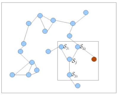
With reference to Figure 1, consider a network with J nodes modeled by an undirected graph

com-Figure 1: Network example where connectivity among nodes, represented by colored circles, is denoted by a line joining them.

municating nodes. Node j∈

J

only communicates with nodes in its one-hop neighborhood (ball)

B

j⊆

J

. The graph

G

is assumed connected, that is, any two nodes in

G

are connected by a (perhaps

multihop) path in

G

. Notice that nodes do not have to be fully connected (any-to-any), and

G

is al-lowed to contain cycles. At every node j∈

J

, a labeled training set

S

j:={(xjn,yjn): n=1, . . . ,Nj}

of size Nj is available, where xjn∈

X

is a p×1 data vector belonging to the input space

X

⊆Rp,

and yjn∈

Y

:={−1,1}denotes its corresponding class label.2

Given

S

j per node j, the goal is to find a maximum-margin linear discriminant function g(x)in

a distributed fashion, and thus enable each node to classify any new input vector x to one of the two classes {−1,1}without communicating

S

j to other nodes j′ 6= j. Potential application scenarios

include but are not limited to the following ones.

Example 1 (Wireless sensor networks). Consider a set of wireless sensors deployed to infer the

presence or absence of a pollutant over a geographical area at any time tn. Sensor j measures

and forms a local binary decision variable yjn∈ {1,−1}, where yjn=1(−1) indicates presence

(absence) of the pollutant at the position vector xj := [xj1, xj2, xj3]T. (Each sensor knows its

position xj using existing self-localization algorithms Langendoen and Reijers, 2003.) The goal

is to have each low-cost sensor improve the performance of local detection achieved based on

S

j ={([xTj,tn]T,yjn): n=1, . . . ,Nj}, and through collaboration with other sensors approach the

global performance attainable if each sensor had available all other sensors data. Stringent power limitations prevent sensor j to send its set

S

jto all other sensors or to an FC, if the latter is available.

If these sensors are acoustic and are deployed to classify underwater unmanned vehicles, divers or submarines, then low transmission bandwidth and multipath effects further discourage incremental communication of the local data sets to an FC (Akyildiz et al., 2005).

Example 2 (Distributed medical databases). Suppose that

S

j are patient data records stored at a

hospital j. Each xjnhere contains patient descriptors (e.g., age, sex or blood pressure), and yjnis a

particular diagnosis (e.g., the patient is diabetic or not). The objective is to automatically diagnose

(classify) a patient arriving at hospital j with descriptor x, using all available data{

S

j}Jj=1, rather

than

S

jalone. However, a nonchalant exchange of database entries(xTjn,yjn)can pose a privacy risk

for the information exchanged. Moreover, a large percentage of medical information may require exchanging high resolution images. Thus, communicating and processing large amounts of high-dimensional medical data at an FC may be computationally prohibitive.

Example 3 (Collaborative data mining). Consider two different government agencies, a local

agency A and a nation-wide agency B, with corresponding databases

S

A and

S

B. Both agencies

are willing to collaborate in order to classify jointly possible security threats. However, lower clear-ance level requirements at agency A prevents agency B from granting agency A open access to

S

B.

Furthermore, even if an agreement granting temporary access to agency A were possible, databases

S

A and

S

Bare confined to their current physical locations due to security policies.

If{

S

j}J_j=1 were all centrally available at an FC, then the global variables w∗and b∗describing

the centralized maximum-margin linear discriminant function g∗(x) =xTw∗+b∗could be obtained by solving the convex optimization problem; see, for example, Sch¨olkopf and Smola (2002, Ch. 7)

{w∗,b∗}=arg min

w,b,{ξjn}

1 2kwk

2

+C J

∑

j=1 Nj

∑

n=1

ξjn

s.t. yjn(wTxjn+b)≥1−ξjn ∀j∈

J

,n=1, . . . ,Nj

ξjn≥0 ∀j∈

J

,n=1, . . . ,Nj

(1)

where the slack variables ξjn account for non-linearly separable training sets, and C is a tunable

positive scalar.

Nonlinear discriminant functions g(x) can also be found along the lines of (1) after mapping vectors xjn to a higher dimensional space

H

⊆RP, with P> p, via a nonlinear transformation

φ:

X

→

H

. The generalized maximum-margin linear classifier in

H

is then obtained after replacing

xjnwithφ(xjn)in (1), and solving the following optimization problem

{w∗,b∗}=arg min

w,b,{ξjn}

1 2kwk

2_+C

∑

J j=1

Nj

∑

n=1

ξjn

s.t. yjn(wTφ(xjn) +b)≥1−ξjn ∀j∈

J

,n=1, . . . ,Nj

ξjn≥0 ∀j∈

J

,n=1, . . . ,Nj.

(2)

Problem (2) is typically tackled by solving its dual. Letting λjn denote the Lagrange multiplier

corresponding to the constraint yjn(wTφ(xjn) +b)≥1−ξjn, the dual problem of (2) is:

max

{λjn} −

1 2

J

∑

j=1 J

∑

i=1 Nj

∑

n=1 Ni

∑

m=1

λjnλimyjnyimφT(xjn)φ(xim) + J

∑

j=1 Nj

∑

n=1

λjn

s.t.

J

∑

j=1 Nj

∑

n=1

λjnyjn=0 (3)

Using the Lagrange multipliersλ∗_jnoptimizing (3), and the Karush-Kuhn-Tucker (KKT) optimality conditions, the optimal classifier parameters can be expressed as

w∗=

J

∑

j=1 Nj

∑

n=1

λ∗

jnyjnφ(xjn),

b∗=yjn−w∗Tφ(xjn) (4)

with xjnin (4) satisfyingλ∗jn∈(0,C). Training vectors corresponding to non-zeroλ∗jn’s constitute

the SVs. Once the SVs are identified, all other training vectors with λ∗_jn=0 can be discarded since they do not contribute to w∗. From this vantage point, SVs are the most informative elements of the training set. Solving (3) does not require knowledge of φ but only inner product values

φT_(x

jn)φ(xim):=K(xjn,xim), which can be computed through a pre-selected positive semi-definite

kernel K :

X

×

X

→R_{; see, for example, Sch¨olkopf and Smola (2002, Ch. 2). Although not} explicitly given, the optimal slack variablesξ∗_jncan be found through the KKT conditions of (2) in terms ofλ∗_jn(Sch¨olkopf and Smola, 2002). The optimal discriminant function can be also expressed in terms of kernels as

g∗(x) =

J

∑

j=1 Nj

∑

n=1

λ∗

jnyjnK(xjn,x) +b∗ (5)

where b∗=yjn−∑Ji=1∑ Ni

m=1λ∗imyimK(xim,xjn) for any SV xjn with λ∗jn∈(0,C). This so-called

kernel trick allows finding maximum-margin linear classifiers in higher dimensional spaces without explicitly operating in such spaces (Sch¨olkopf and Smola, 2002).

The objective here is to develop fully distributed solvers of the centralized problems in (1) and (2) while guaranteeing performance approaching that of a centralized equivalent SVM. Although incremental solvers are possible, the size of information exchanges required might be excessive, especially if the number of SVs per node is large (Flouri et al., 2008; Lu et al., 2008). Recall that exchanging all local SVs among all nodes in the network several times is necessary for incremental DSVMs to approach the optimal centralized solution. Moreover, incremental schemes require a Hamiltonian cycle in the network to be identified in order to minimize the communication overhead. Computing such a cycle is an NP-hard task and in most cases a sub-optimal cycle is used at the expense of increased communication overhead. In other situations, communicating SVs directly might be prohibited because of the sensitivity of the information bore, as already mentioned in Examples 2 and 3.

3. Distributed Linear Support Vector Machine

This section presents a reformulation of the maximum-margin linear classifier problem in (1) to an equivalent distributed form, which can be solved using the alternating direction method of multipli-ers (ADMoM) outlined in Appendix A. (For detailed exposition of the ADMoM, see, for example, Bertsekas and Tsitsiklis, 1997.)

To this end, consider replacing the common (coupling) variables (w,b) in (1) with auxiliary per-node variables{(wj,bj)}J_j=1, and adding consensus constraints to force these variables to agree

reformulation of (1) becomes

min

{wj,bj,ξjn}

1 2

J

∑

j=1

wj 2 +JC J

∑

j=1 Nj

∑

n=1

ξjn

s.t. yjn(wTjxjn+bj)≥1−ξjn ∀j∈

J

,n=1, . . . ,Nj

ξjn≥0 ∀j∈

J

,n=1, . . . ,Nj

wj=wi,bj=bi ∀j∈

J

,i∈

B

j.

(6)

From a high-level view, problem (6) can be solved in a distributed fashion because each node j can optimize only the j-dependent terms of the cost, and also meet all the consensus constraints

wj=wi,bj=bi, by exchanging messages only with nodes i in its neighborhood

B

j. What is more,

network connectivity ensures that consensus in neighborhoods enables network-wide consensus. And thus, as the ensuing lemma asserts, solving (6) is equivalent to solving (1) so long as the network remains connected.

Lemma 1 If{(wj,bj)}J_j=1 denotes a feasible solution of (6), and the graph

G

is connected, then problems (1) and (6) are equivalent, that is, wj =w and bj=b ∀j=1, . . . ,J, where (w,b)is a feasible solution of (1).

Proof See Appendix B.

To specify how (6) can be solved using the ADMoM, define for notational brevity the aug-mented vector vj:= [wTj,bj]T, the augmented matrix Xj:= [[xj1, . . . ,xjNj]

T_,1

j], the diagonal label

matrix Yj:=diag([yj1, . . . ,yjNj]), and the vector of slack variablesξj:= [ξj1, . . . ,ξjNj]

T_{. With these}

definitions, it follows readily that wj= (Ip+1−Πp+1)vj, whereΠp+1is a(p+1)×(p+1)matrix

with zeros everywhere except for the(p+1,p+1)-st entry, given by[Πp+1](p+1)(p+1)=1. Thus, problem (6) can be rewritten as

min

{vj,ξj,ωji}

1 2

J

∑

j=1

vT_j(Ip+1−Πp+1)vj +JC J

∑

j=1 1T_jξ_j

s.t. YjXjvj1j−ξj ∀j∈

J

ξj0j ∀j∈

J

vj=ωji,ωji=vi ∀j∈

J

,∀i∈

B

j

(7)

where the redundant variables{ωji}will turn out to facilitate the decoupling of the classifier

pa-rameters vj at node j from those of their neighbors at neighbors i∈

B

j.

As in the centralized case, problem (7) will be solved through its dual. Toward this objective, let

αji1 (αji2) denote the Lagrange multipliers corresponding to the constraint vj=ωji (respectively

ωji=vi), and consider what we term surrogate augmented Lagrangian function

L

({vj},{ξj},{ωji},{αjik}) =

1 2

J

∑

j=1

vT_j(Ip+1−Πp+1)vj+JC J

∑

j=1 1T_jξ_j+

J

∑

j=1i∈

∑

Bj

αT

ji1(vj−ωji)

+

J

∑

j=1i

∑

∈Bj

αT

ji2(ωji−vi)+

η

2

J

∑

j=1i∈

∑

Bj

vj−ωji

2 +η 2 J

∑

j=1i

∑

∈Bj

ωji−vi

2

where the adjective “surrogate” is used because

L

does not include the set of constraints

W

:=

{YjXjvj 1j−ξj, ξj 0j}, and the adjective “augmented” because

L

includes two quadratic

terms (scaled by the tuning constantη>0) to further regularize the equality constraints in (7). The role of these quadratic terms||vj−ωji||2and||ωji−vi||2is twofold: (a) they effect strict convexity

of

L

with respect to (w.r.t.) ωji, and thus ensure convergence to the unique optimum of the global

cost (whenever possible), even when the local costs are convex but not strictly so; and (b) through the scalarη, they allow one to trade off speed of convergence for steady-state approximation error (Bertsekas and Tsitsiklis, 1997, Ch. 3).

Consider now solving (7) iteratively by minimizing

L

in a cyclic fashion with respect to one set of variables while keeping all other variables fixed. The multipliers {αji1,αji2}must be also

updated per iteration using gradient ascent. The iterations required per node j are summarized in the following lemma.

Lemma 2 The distributed iterations solving (7) are

{vj(t+1),ξj(t+1)} = arg min {vj,ξj}∈W

L

({vj},{ξj},{ωji(t)},{αjik(t)}), (9)

{ωji(t+1)} = arg min

{ωji}

L

({vj(t+1)},{ξj(t+1)},{ωji},{αjik(t)}), (10)

αji1(t+1) = αji1(t) +η(vj(t+1)−ωji(t+1)) ∀j∈

J

,∀i∈

B

j, (11)

αji2(t+1) = αji2(t) +η(ωji(t+1)−vi(t+1)) ∀j∈

J

,∀i∈

B

j. (12)

and correspond to the ADMoM solver reviewed in Appendix A.

Proof See Appendix C.

Lemma 2 links the proposed DSVM design with the convergent ADMoM solver, and thus en-sures convergence of the novel MoM-DSVM to the centralized SVM classifier. However, for the particular problem at hand it is possible to simplify iterations (9)-(12). Indeed, simple inspection of (8) confirms that with all other variables fixed, the cost in (10) is linear-quadratic inωji; hence,

ωji(t+1) can be found in closed form per iteration, and the resulting closed-form expression can

be substituted back to eliminate ωji from

L

. Furthermore, Appendix D shows that the two sets

of multipliersαji1 andαji2 can be combined into one setαj after appropriate initialization of the

iterations (11) and (12), as asserted by the following lemma.

Lemma 3 Selectingαji1(0) =αji2(0) =0(p+1)×1as initialization∀j∈

J

,∀i∈

B

j, iterations

(9)-(12) reduce to

{vj(t+1),ξj(t+1)} = arg min {vj,ξj}∈W

L

′({vj},{ξj},{vj(t)},{αj(t)}), (13)

αj(t+1) = αj(t) +

η

2_i

∑

_∈B

j

whereαj(t):=∑i∈Bjαji1(t), and

L

′ _{is given by}

L

′({vj},{ξj},{vj(t)},{αj(t)}) =

1 2

J

∑

j=1

vT_j(Ip+1−Πp+1)vj+JC J

∑

j=1 1T_jξ_j

+2

J

∑

j=1

αT

j(t)vj+η J

∑

j=1i∈

∑

Bj

vj−

1

2[vj(t) +vi(t)] 2 . (15)

Proof See Appendix D.

The optimization problem in (13) involves the reduced Lagrangian

L

′ in (15), which is linear-quadratic in vj andξj. In addition, the constraint set

W

is linear in these variables. To solve

this constrained minimization problem through its dual, letλj:= [λj1, . . . ,λjNj]

T _{denote Lagrange}

multipliers per node corresponding to the constraints YjXjvj1j−ξj. Solving the dual of (13)

yields the optimal λj at iteration t+1, namely λj(t+1), as a function of vj(t) andαj(t); while

the KKT conditions provide expressions for vj(t+1)as a function ofαj(t), and the optimal dual

variablesλj(t+1). Notwithstanding, the resultant iterations are decoupled across nodes. These

iterations and the associated convergence guarantees can be summarized as follows.

Proposition 1 Consider the per node iteratesλj(t), vj(t)andαj(t), given by

λj(t+1) =arg max

λj: 0jλjJC1j −1

2λ

T

jYjXjU−1j X T jYjλj+

1j+YjXjU−1j fj(t)

T

λj, (16)

vj(t+1) =U−1j

XT_jYjλj(t+1)−fj(t)

, (17)

αj(t+1) =αj(t) +

η

2_i∈

∑

_B

j

[vj(t+1)−vi(t+1)] (18)

where Uj:= (1+2η|

B

j|)Ip+1−Πp+1, fj(t):=2αj(t)−η∑i∈Bj[vj(t) +vi(t)],η>0, and arbitrary initialization vectorsλj(0), vj(0), andαj(0) =0(p+1)×1. The iterate vj(t)converges to the solution of (7), call it v∗, as t→∞; that is, limt→∞vj(t) =v∗.

Proof See Appendix E.

Similar to the centralized SVM algorithm, if[λj(t)]n6=0, then[xTjn,1]T is an SV. Findingλj(t+

1)as in (16) requires solving a quadratic optimization problem similar to the one that a centralized SVM would solve, for example, via a gradient projection algorithm or an interior point method; see for example, Sch¨olkopf and Smola (2002, Ch. 6). However, the number of variables involved in (16) per iteration per node is considerably smaller when compared to its centralized counterpart, namely Nj versus∑Jj=1Nj. Also, the optimal local slack variables ξ∗j can be found via the KKT

conditions for (13).

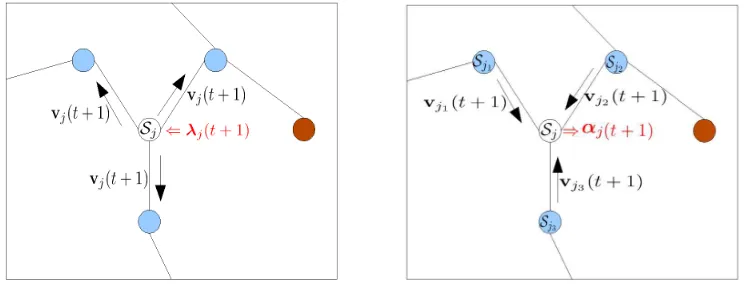
The ADMoM-based DSVM (MoM-DSVM) iterations (16)-(18) are summarized as Algorithm 1, and are illustrated in Figure 2. All nodes have available JC andη. Also, every node computes its local Nj×Njmatrix YjXjU−1j XTjYj, which remains unchanged throughout the entire algorithm.

At iteration t+1, node j computes vector fj(t)locally to obtain its localλj(t+1)via (16). Vector

λj(t+1) together with the local training set

S

j are used at node j to compute vj(t+1)via (17).

Next, node j broadcasts its newly updated local estimates vj(t+1) to all its one-hop neighbors i∈

B

j. Iteration t+1 resumes when every node updates its localαj(t+1) vector via (18). Note

that at any given iteration t of the algorithm, each node j can evaluate its own local discriminant function g(_jt)(x)for any vector x∈

X

as

g(_jt)(x) = [xT,1]vj(t) (19)

which from Proposition 1 is guaranteed to converge to the same solution across all nodes as t→∞. Simulated tests in Section 5 will demonstrate that after a few iterations the classification perfor-mance of (19) outperforms that of the local discriminant function obtained based on the local train-ing set alone. The effect ofηon the convergence rate of MoM-DSVM will be tested numerically in Section 5.

Figure 2: Visualization of iterations (16)-(18): (left) every node j∈

J

computesλj(t+1)to obtain vj(t+1), and then broadcasts vj(t+1)to all neighbors i∈

B

j; (right) once every node

j∈

J

has received vi(t+1)from all i∈

B

j, it computesαj(t+1).

Remark 1 The messages exchanged among neighboring nodes in the MoM-DSVM algorithm cor-respond to local estimates vj(t), which together with the local multiplier vectors αj(t), convey sufficient information about the local training sets to achieve consensus globally. Per iteration and per node a message of fixed size(p+1)×1 is broadcasted (vectorsαjare not exchanged among nodes.) This is to be contrasted with incremental DSVM algorithms in, for example, Lu et al. (2008), Flouri et al. (2006) and Flouri et al. (2008), where the size of the messages exchanged between neighboring nodes depends on the number of SVs found at each incremental step. Although the SVs of each training set may be few, the overall number of SVs may remain large, thus consuming considerable power when transmitting SVs from one node to the next.

Algorithm 1 MoM-DSVM

Require: Randomly initialize vj(0), andαj(0) =0(p+1)×1for every j∈

J

1: for t=0,1,2, . . .do

2: for all j∈

J

do

3: Computeλj(t+1)via (16). 4: Compute vj(t+1)via (17). 5: end for

6: for all j∈

J

do

7: Broadcast vj(t+1)to all neighbors i∈

B

j. 8: end for

9: for all j∈

J

do

10: Computeαj(t+1)via (18). 11: end for

12: end for

node that fails, say jo∈

J

, does not correspond to a cut-vertex of

G

. In this case, the operational network graph

G

o:=

G

−joremains connected, and thus surviving nodes can percolate information throughout

G

o. Of course,

S

jo will not participate in training the SVM. If jo is a cut-vertex of

G

, the algorithm will remain operational in each connected component of the resulting sub-graph

G

o, reaching consensus among nodes in each of the connected components.

3.1 Online Distributed Support Vector Machine

In many distributed learning tasks data arrive sequentially, and possibly asynchronously. In addition, the processes to be learned may change with time. In such cases, training examples need to be added or removed from each local training set

S

j. Training sets of increasing of decreasing size can be

expressed in terms of time-varying augmented data matrices Xj(t), and corresponding label matrices Yj(t). An online version of DSVM is thus well motivated when a new training example xjn(t)

along with its label yjn(t)acquired at time t are incorporated into Xj(t)and Yj(t), respectively. The

corresponding modified iterations are given by (cf. (16)-(18))

λj(t+1) = arg max

λj: 0j(t+1)λjJC1j(t+1) −1

2λ

T

jYj(t+1)Xj(t+1)U−1j Xj(t+1)TYj(t+1)λj

+1j−Yj(t+1)Xj(t+1)U−1j fj(t)

T

λj, (20)

vj(t+1) = U−1j Xj(t+1)TYj(t+1)λj(t+1)−2αj(t) +η

∑

i∈Bj

[vj(t) +vi(t)]

!

, (21)

αj(t+1) = αj(t) +

η

2_i

∑

_∈B

j

[vj(t+1)−vi(t+1)]. (22)

Note that the dimensionality ofλjmust vary to accommodate the variable number of

S

jelements

at every time instant t. The online MoM-DSVM classifier is summarized as Algorithm 2. For this algorithm to run, no conditions need to be imposed on how the sets

S

j(t)increase or decrease. Their

Algorithm 2 Online MoM-DSVM

Require: Randomly initialize vj(0), andαj(0) =0(p+1)×1for every j∈

J

. 1: for t=0,1,2, . . .do

2: for all j∈

J

do

3: Update Yj(t+1)Xj(t+1)U−1j Xj(t+1)TYj(t+1). 4: Computeλj(t+1)via (20).

5: Compute vj(t+1)via (21). 6: end for

7: for all j∈

J

do

8: Broadcast vj(t+1)to all neighbors i∈

B

j. 9: end for

10: for all j∈

J

do

11: Computeαj(t+1)via (22). 12: end for

13: end for

the parameters ηand C can also become time-dependent. The effect of these parameters will be discussed in Section 5.

Intuitively speaking, if the training sets remain invariant across a sufficient number of time instants, vj(t) will closely track the optimal linear classifier. Rigorous convergence analysis of

Algorithm 2 for any given rate of change of the training set goes beyond the scope of this work. Simulations will however demonstrate that the modified iterations in (20)-(22) are able to track changes in the training sets even when these occur at every time instant t.

Remark 3 Compared to existing centralized online SVM alternatives in, for example, Cauwen-berghs and Poggio (2000) and Fung and Mangasarian (2002), the online MoM-DSVM algorithm of this section allows seamless integration of both distributed and online processing. Nodes with training sets available at initialization and nodes that are acquiring their training sets online can be integrated to jointly find the maximum-margin linear classifier. Furthermore, whenever needed, the online MoM-DSVM can return a partially trained model constructed with examples available to the network at any given time. Likewise, elements of the training sets can be removed without hav-ing to restart the MoM-DSVM algorithm. This feature also allows adapthav-ing MoM-DSVM to jointly operate with algorithms that account for concept drift (Klinkenberg and Joachims, 2000). In the classification context, concept drift defines a change in the true classification boundaries between classes. In general, accounting for concept drift requires two main steps, which can be easily han-dled by the online MoM-DSVM: (i) acquisition of updated elements in the training set that better describe the current concept; and (ii) removal of outdated elements from the training set.

4. Distributed Nonlinear Support Vector Machine

(16)-(18) to be carried in

H

. As the dimensionality P of

H

increases, the local computation and communication complexities become increasingly prohibitive.

Our approach to mitigate this well-known “curse of dimensionality” is to enforce consensus of the local discriminants g∗_j on a subspace of reduced rank L<P. To this end, we project the

consensus constraints corresponding to (2) and consider the optimization problem (cf. (6))

min

{wj,bj,ξj}

1 2

J

∑

j=1

kwjk2+JC J

∑

j=1 1T_jξ_j

s.t. Yj(Φ(Xj)wj+1jbj)1j−ξj ∀j∈

J

ξ_j0j ∀j∈

J

Gwj=Gwi ∀j∈

J

,i∈

B

j bj=bi ∀j∈

J

,i∈

B

j

(23)

where Φ(Xj):= [φ(xj1), . . . ,φ(xjNj)]

T_{, and G := [}φ₍χ

1), . . . ,φ(χL)]T is a fat L×P matrix

com-mon to all nodes with preselected vectors{χ_l}L

l=1specifying its rows. Eachχl∈

X

corresponds to a

φ(χ_l)∈

H

, which at the optimal solution{w∗_j,b∗_j}J

j=1of (23), satisfiesφT(χl)w∗1=· · ·=φT(χl)w∗J=

φT_(χ

l)w∗. The projected constraints{Gwj=Gwi}along with{bj =bi}force all nodes to agree

on the value of the local discriminant functions g∗_j(χ_l)at the vectors{χ_l}L

l=1, but not necessarily for

all x∈

X

. This is the price paid for reducing the computational complexity of (23) to an affordable level. Clearly, the choice of vectors {χ_l}L

l=1, their number L, and the local training sets

S

j

deter-mine how similar the local discriminant functions g∗_j are. If G=IP, then (23) reduces to (6), and

g∗₁(x) =. . .=g∗_J(x) =g∗(x),∀x∈

X

, but the high dimensionality challenge appears. At the end of

this section, we will provide different design choices for{χ_l}L

l=1, and test them via simulations in

Section 5.

Because the cost in (23) is strictly convex w.r.t. wj, it guarantees that the set of optimal vectors {w∗_j}is unique even when G is a ‘fat’ matrix (L<P) and/or ill-conditioned (Bertsekas, 1999, Prop.

5.2.1). As in (2), having{w∗_j}known is of limited use, since the mappingφmay be unknown, or if known, evaluating vectorsφ(x)may entail an excessive computational cost. Fortunately, the result-ing discriminant function g∗_j(x)admits a reduced-complexity solution because it can be expressed in terms of kernels, as shown by the following theorem.

Theorem 4 For every positive semi-definite kernel K(·,·), the discriminant functions g∗_j(x) =

φT_(x)w∗

j+b∗j with{w∗j,b∗j}denoting the optimal solution of (23), can be written as

g∗_j(x) =

Nj

∑

n=1

a∗_jnK(x,xjn) + L

∑

l=1

c∗_jlK(x,χ_l) +b∗_j,∀j∈

J

(24)

where{a∗_jn}and{c∗_jl}are real-valued scalar coefficients.

Proof See Appendix F.

The space of functions gjdescribed by (24) is fully determined by the span of the kernel function K(·,·) centered at training vectors {xjn,n=1, . . . ,Nj} per node, and also at the vectors {χl}Ll=1

naturally constrained by the corresponding

S

j. Theorem 1 also reveals the effect of{χl}Ll=1on the {g∗_j}. By introducing vectors{χ_l}L

l=1common to all nodes, a subset of basis functions common to

all local functional spaces is introduced a fortiori. Coefficients a∗_jnand c∗_jlare found so that all local discriminants g∗_j agree on their values at points{χ_l}L

l=1. Intuitively, at every node these coefficients

summarize the global information available to the network.

Theorem 1 is an existence result whereby each nonlinear discriminant function g∗_j is expressible in terms of

S

j and{χl}Ll=1. However, finding the coefficients a∗jn, c∗jland b∗j in a distributed fashion

remains an issue. Next, it is shown that these coefficients can be obtained iteratively by applying the ADMoM solver to (23).

Similar to (7), introduce auxiliary variables{ωji}({ζji}) to decouple the constraints Gwj=Gwi

(bj=bi) across nodes, andαjik (βjik) denote the corresponding Lagrange multipliers (cf. (8)). The

surrogate augmented Lagrangian for problem (23) is then

L

({wj},{ξj},{ωji},{αjik},{ζji},{βjik}) =

1 2

J

∑

j=1

kwjk2+JC J

∑

j=1 1T_jξ_j+

J

∑

j=1i∈

∑

Bj

αT

ji1(Gwj−ωji)

+

J

∑

j=1i∈

∑

Bj

αT

ji2(ωji−Gwi)+ J

∑

j=1i∈

∑

Bj

βji1(bj−ζji)+ J

∑

j=1i

∑

∈Bj

βji2(ζji−bi)

+η 2

J

∑

j=1i

∑

∈Bj

Gwj−ωji

2 +η 2 J

∑

j=1i∈

∑

Bj

ωji−Gwi

2 +η 2 J

∑

j=1i

∑

∈Bj

bj−ζji

2 +η 2 J

∑

j=1i∈

∑

Bj

ζji−bi

2

.

Following the steps of Lemma 2, and with{αjik}and{βjik} initialized at zero, the ADMoM

iterations take the form

{wj(t+1),bj(t+1),ξj(t+1)}=arg min {wj,bj,ξj}∈W

L

′({wj},{bj},{ξj},{αj(t)},{βj(t)}), (25)

αj(t+1) =αj(t) +

η

2_i

∑

_∈B

j

G[wj(t+1)−wi(t+1)], (26)

βj(t+1) =βj(t) +

η

2_i∈

∑

_B

j

[bj(t+1)−bi(t+1)] (27)

where

L

′ _{is defined similar to (8),α}

j(t)as in Lemma 3, andβj(t):=∑i∈Bjβji1(t). The ADMoM

iterations (25)-(27) will not be explicitly solved since iterates wj(t) lie in the high-dimensional

space

H

. Nevertheless, our objective is not to find w∗_j, but rather the discriminant function g∗_j(x). To this end, letΓ:= [χ₁, . . . ,χ_L]T_{, and define the kernel matrices with entries}

[K(Xj,Xj)]n,m:=K(xjn,xjm), (28)

[K(Xj,Γ)]n,l :=K(xjn,χl), (29)

[K(Γ,Γ)]l,l′ :=K(χ_l,χ_l′). (30)

From Theorem 1 it follows that each local update g(_jt)(x) =φT(x)wj(t) +bj(t)admits per iteration t

a solution expressed in terms of kernels. The latter is specified by the coefficients{ajn(t)},{cjl(t)}

Proposition 2 Letλj:= [λj1, . . . ,λjNj]

T _{denote the Lagrange multiplier corresponding to the}

con-straint Yj(Φ(Xj)wj+1jbj)1j−ξj, andwej(t):=Gwj(t). The local discriminant function g(_jt)(x) at iteration t is

g(_jt)(x) =

Nj

∑

n=1

ajn(t)K(x,xjn) + L

∑

l=1

cjl(t)K(x,χl) +bj(t) (31)

where aj(t):= [aj1(t), . . . ,ajNj(t)] T_{, c}

j(t):= [cj1(t), . . . ,cjL(t)]T, and bj(t)are given by

aj(t):=Yjλj(t), (32)

cj(t):=2η|

B

j|Ue−1_j [K(Γ,Γ)fj(t)−K(Γ,Xj)Yjλj(t)]−efj(t), (33) bj(t):=

1 2η|

B

j|

1T_jYjλj(t)−hj(t)

(34)

withλj(t)denoting the vector multiplier update available at iteration t,Uej:=IL+2η|

B

j|K(Γ,Γ),

efj(t):=2αj(t)−η∑i∈Bj[wej(t) +wei(t)]and hj(t):=2βj(t)−η∑i∈Bj[bj(t) +bi(t)].

Proof See Appendix G.

Proposition 2 asserts that in order to find aj(t), cj(t)and bj(t)in (32), (33) and (34), it suffices

to obtainλj(t),wej(t), bj(t),αj(t), andβj(t). Note that finding the L×1 vectorwej(t)from wj(t)

incurs complexity of order O(L). The next proposition shows how to iteratively updateλj(t),wej(t), bj(t),αj(t), andβj(t)in a distributed fashion.

Proposition 3 The iteratesλj(t),wej(t), bj(t),αj(t)andβj(t)can be obtained as

λj(t+1) =arg max

λj: 0jλjJC1j −1

2λ

T jYj

K(Xj,Xj)−Ke(Xj,Xj) + 1j1Tj

2η|

B

j|

Yjλj+1Tjλj

−

efT_j(t)K(Γ,Xj)−Ke(Γ,Xj)

+hj(t)

1T

2η|

B

j|

Yjλj, (35)

e

wj(t+1) =

h

K(Γ,Xj)−Ke(Γ,Xj)

i

Yjλj(t+1)−

h

K(Γ,Γ)−Ke(Γ,Γ)iefj(t), (36)

bj(t+1) =

1 2η|

B

j|

1T_jYjλj(t+1)−hj(t)

, (37)

αj(t+1) =αj(t) +

η

2_i∈

∑

_B

j

[wej(t+1)−wei(t+1)], (38)

βj(t+1) =βj(t) +

η

2_i

∑

_∈B

j

[bj(t+1)−bi(t+1)] (39)

where Ke(Z,Z′):=2η|

B

j|K(Z,Γ)Ue−1j K(Γ,Z′). With arbitrary initialization λj(0), wej(0), and bj(0); and αj(0) =0L×1 andβj(0) =0, the iterates {ajn(t)}, {cjl(t)} and{bj(t)} in (32), (33) and (34) converge to{a∗_jn},{c∗_jl}and{b∗_j}in (24), as t→∞,∀j∈

J

,n=1, . . . ,Nj, and l=1, . . . ,L.

Algorithm 3 MoM-NDSVM

Require: Randomly initializewej(0)and bj(0); andαj(0) =0L×1andβj(0) =0 for every j∈

J

. 1: for t=0,1,2, . . .do

2: for all j∈

J

do

3: Computeλj(t+1)via (35). 4: Computewej(t+1)via (36). 5: Compute bj(t+1)via (37). 6: end for

7: for all j∈

J

do

8: Broadcastwej(t+1)and bj(t+1)to all neighbors i∈

B

j. 9: end for

10: for all j∈

J

do

11: Computeαj(t+1)via (38). 12: Computeβj(t+1)via (39).

13: Compute aj(t), cj(t)and bj(t)via (32), (33) and (34), respectively. 14: end for

15: end for

The iterations comprising the ADMoM-based non-linear DSVM (MoM-NDSVM) are summa-rized as Algorithm 3. It is important to stress that Algorithm 3 starts by having all nodes agree on the common quantitiesΓ, JC, η, and K(·,·). Also, each node computes its local kernel matrices as in (28)-(30), which remain unchanged throughout. Subsequently, Algorithm 3 runs in a manner analogous to Algorithm 1, with the difference that every node communicates an(L+1)×1 vector (instead of(p+1)×1) for its neighbors to receivewej(t)and bj(t).

4.1 On the Optimality of NDSVM and the Selection of Common Vectors

By construction, Algorithm 3 produces local discriminant functions whose predictions for{χ_l}L l=1

are the same for all nodes in the network; that is, g∗₁(χ_l) =. . .=g∗_J(χ_l) =g∗(χ_l)for l=1, . . . ,L,

where g∗(χ_l) =φT_(χ

l)w∗+b∗, and {w∗,b∗} are the optimal solution of the centralized problem

(2). Viewing{χ_l}L

l=1 as a classification query, the proposed MoM-NDSVM algorithm can be

im-plemented as follows. Having this query presented at any node j entailing a set of unlabeled vectors

{χ_l}L

l=1, the novel scheme first percolates{χl}Ll=1throughout the network.3 Problem (23) is

subse-quently solved in a distributed fashion using Algorithm 3. Notice that in this procedure no database information is shared.

Although optimal in the sense of being convergent to its centralized counterpart, the algorithm just described needs to be run for every new classification query. Alternatively, one can envision procedures to find discriminant functions in a distributed fashion that classify new queries without having to re-run the distributed algorithm. The key is to pre-select a fixed set {χ_l}L

l=1 for which g∗ in (5) is (approximately) equivalent to g∗_j in (24) for all j∈

J

. From Theorem 1, we know that all local functions g∗_j share a common space spanned by theχ_l-induced kernels{K(·,χ_l)}. If the space

H

where g∗lies is finite dimensional, for example, when adopting linear or polynomial

3. Percolating{χ}L

l=1in a distributed fashion through the network can be carried in a finite number of iterations at most

kernels in (5), one can always find a finite-size set {χ_l}L

l=1 such that the space spanned by the

set of kernels{K(·,χ_l)} contains

H

, and thus g∗₁(x) =. . .=g∗_J(x) =g∗(x) ∀x∈

X

(Predd et al., 2006). Indeed, when using linear kernels, the MoM-NDSVM developed here boils down to the MoM-DSVM developed in Section 3 for a suitable finite-size set{χ_l}L

l=1.

In general, however, the space spanned by{K(·,χ_l)}may have lower dimensionality than

H

; thus, local functions g∗_j do not coincide at every point. In this case, MoM-NDSVM finds local approximations to the centralized g∗which accommodate information available to all nodes. The degree of approximation depends on the choice of{χ_l}L

l=1. In what follows, we describe two

alter-natives to constructing such a set{χ_l}L l=1.

• Grid-based designs. Consider every entry k of the training vectors {xjn}, and form the

intervals

I

k := [xmin_k ,xmax_k ], k=1, . . . ,p, where x_kmin :=minj∈J,n=1,...,Nj[xjn]k and x max k :=

maxj∈J,n=1,...,Nj[xjn]k. Take for convenience L=M

p_{, and partition uniformly each}

_I

k to

ob-tain a set of M equidistant points

Q

k :={qk1, . . . ,qkM}. The set{χl}Ll=1 can be formed by

taking all Mp possible vectors with entries drawn from the Cartesian product

Q1

×. . . ,×

Q

p.

One possible set we use for generating the{χ_l}L

l=1 vectors is obtained by selecting the k-th

entry of the l-th vector as[χ_l]k=q_k, l Mk−1mod M

+1, where l=1, . . . ,M

p_{and k=1, . . . ,p. In}

this case, MoM-NDSVM performs a global consensus step on the entry-wise maxima and minima of the training vectors{xjn}. Global consensus on the entry-wise maxima and

min-ima can be computed exactly in a finite number of iterations equal to at most the diameter of the graph

G

.

• Random designs. Once again, we consider every entry k of the training vectors{xjn}.

MoM-NDSVM starts by performing a consensus step on the entry-wise maxima and minima of the local training vectors {xjn}. The set {χl}Ll=1 is formed by drawing elements χl randomly

from a uniform p-dimensional distribution with extreme points per entry given by the extreme points xmin_k and xmax_k , k=1, . . . ,p. To agree on the set{χ_l}L

l=1, all nodes in the network are

assumed to share a common seed used to initialize the random sampling algorithms.

As mentioned earlier, the number of points L affects how close local functions are to each other as well as to the centralized one. The choice of L also depends on the kernel used, prior knowledge of the discriminant function, and the available local training data Nj. Increasing L guarantees that

local functions will be asymptotically close to each other regardless of Nj; however, the

commu-nication cost and computational complexity per node will increase according to L [cf. Algorithm 3]. On the other hand, a small L reduces the communication overhead at the price of increasing the disagreement among the g∗_j’s. This trade-off will be further explored in the ensuing section through simulated tests.

5. Numerical Simulations

5.1 Linear Classifiers

In this section, we present experiments on synthetic and real data to illustrate the performance of our distributed method for training linear SVMs.

5.1.1 TESTCASE1: SYNTHETICTRAININGSET

Consider a randomly generated network with J=30 nodes. The network is connected with algebraic connectivity 0.0448 and average degree per node 3.267. Each node acquires labeled training exam-ples from two different classes

C1

and

C2

with corresponding labels y1=1 and y2=−1. Classes

C1

and

C2

are equiprobable and consist of random vectors drawn from a two-dimensional Gaussian distribution with common covariance matrixΣ= [1,0; 0,2], and mean vectors m1 = [−1, −1]T

and m2= [1,1]T, respectively. Each local training set

S

jconsists of Nj=N=10 labeled examples

and was generated by: (i) randomly choosing class

C

k, k=1,2; and, (ii) randomly generating a

la-beled example(xT_jn,yjn=

C

k)with xjn∼

N

(mk,Σ). Thus, the global training set contains JN=300

training examples. Likewise, a test set

STest

:={(exn,eyn), n=1, . . . ,NT}with NT =600 examples,

drawn as in (i) and (ii), is used to evaluate the generalization performance of the classifiers. The Bayes optimal classifier for this 2-class problem is linear (Duda et al., 2002, Ch. 2), with risk

RBayes=0.1103. The empirical risk of the centralized SVM in (1) is defined as

Rcentral_emp := 1

NT NT

∑

n=1

1

2|eyn−yˆn|

where ˆynis the predicted label forexn. The average empirical risk of the MoM-DSVM algorithm as

a function of the number of iterations is defined as

Remp(t):= 1

JNT J

∑

j=1 NT

∑

n=1

1

2|eyn−yˆjn(t)| (40)

where ˆyjn(t) is the label prediction at iteration t and node j forxen, n=1, . . . ,NT using the SVM

parameters in vj(t). The average empirical risk of the local SVMs across nodes Rlocalemp is defined as

in (40) with ˆyjnfound using only locally-trained SVMs.

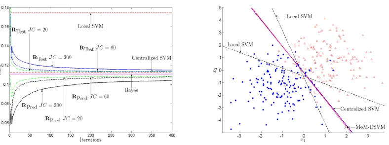
Figure 3 (left) depicts the risk of the MoM-DSVM algorithm as a function of the number of iterations t for different values of JC. In this test, η=10 and a total of 500 Monte Carlo runs are performed with randomly drawn local training and test sets per run. The centralized and local empirical risks with C=10 are included for comparison. The average local prediction performance is also evaluated. Clearly, the risk of the MoM-DSVM algorithm reduces as the number of iterations increases, quickly outperforming local-based predictions and approaching that of the centralized benchmark. To further visualize this test case, Figure 3 (right) shows the global training set, along with the linear discriminant functions found by the centralized SVM and the MoM-DSVM at two different nodes after 400 iterations with JC=20 andη=10. Local SVM results for two different nodes are also included for comparison.

5.1.2 TESTCASE2: MNIST TRAININGSET

Figure 3: Evolution of the test error(RTest)and prediction error(RPred)of MoM-DSVM for a

two-class problem using synthetic data and a network with J=30 nodes. Centralized SVM performance and average local SVMs performance are also plot for comparison (left). Decision boundary comparison among MoM-DSVM, centralized SVM and local SVM results for synthetic data generated from two Gaussian classes (right).

experiment each image is vectorized to a 784 by 1 vector. In particular, we take 5,900 training samples per digit, and a test set of 1,000 samples per digit. Both training and test sets used are as given by the MNIST database, that is, there is no preprocessing of the data. For simulations, we consider two randomly generated networks with J=25, algebraic connectivity 3.2425, and average degree per node 12.80; and J=50 nodes, algebraic connectivity 1.3961, and average degree per node 15.92. The training set is equally partitioned across nodes, thus every node in the network with J=25 has Nj=472 training vectors, and every node in the network with J=50 has Nj=236

samples. The distribution of samples across nodes influences the training phase of MoM-DSVM. For example, if data per node are biased toward one particular class, then the training phase may require more iterations to percolate appropriate information across the network. In the simulations, we consider the two extreme cases: (i) training data are evenly distributed across nodes, that is, every node has the same number of examples from digit 2 and from digit 9; and, (ii) highly biased local data, that is, every node has data corresponding to a single digit; thus, a local binary classifier cannot be constructed.

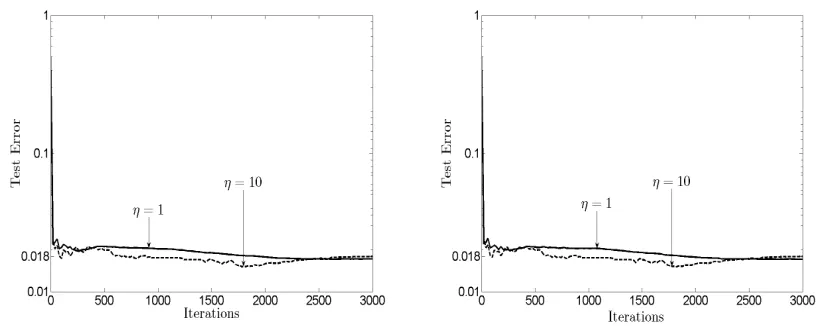
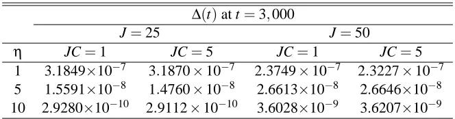
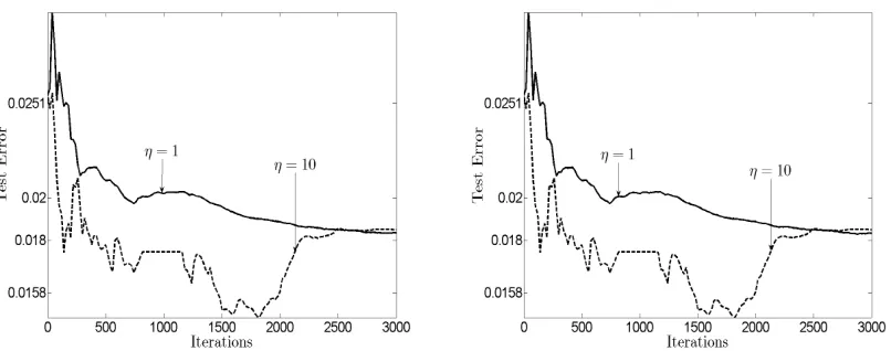
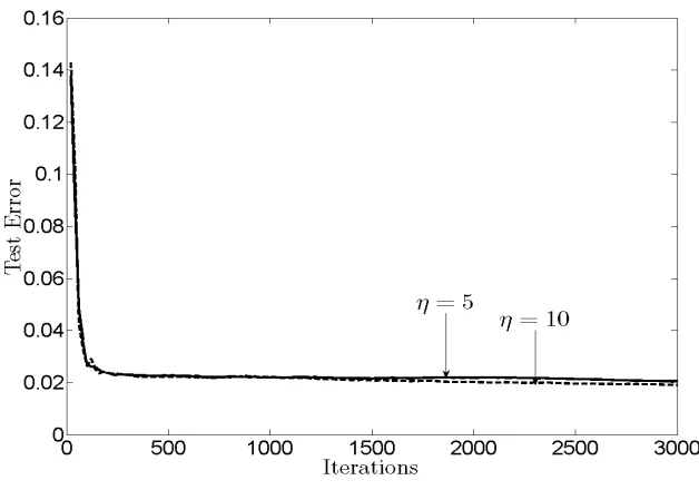
The figures in this section correspond to one run of the MoM-DSVM for a network with noise-less communication links. Figure 4 shows the evolution of the test error for the network with 25 nodes and highly biased local data. Likewise, Figure 5 shows the evolution of the test error for the network with 50 nodes and highly biased local data. Different values for the penalties JC and

Figure 4: Evolution of the test error(RTest)of MoM-DSVM, with penalty coefficients JC=1 (left)

and JC=5 (right), for a two-class problem using digits 2 and 9 from the MNIST data set unevenly distributed across nodes, and a network with J=25 nodes.

Figure 5: Evolution of the test error(RTest)of MoM-DSVM, with penalty coefficients JC=1 (left)

and JC=5 (right), for a two-class problem using digits 2 and 9 from the MNIST data set unevenly distributed across nodes, and a network with J=50 nodes.

Next, the dispersion of the solutions after 3,000 iterations for different values of ηis tested. For our experiment, dispersion refers to how similar are the local vj(t)at every node. The

mean-squared error (MSE) of the solution across nodes is defined as∆(t):=1_J∑J_j=1||vj(t)−¯v(t)||2where

¯v(t):= 1 J∑

J

j=1vj(t). Table 1 shows∆(t)at t=3,000 for different values ofηand JC. Note that