R E S E A R C H A R T I C L E
Open Access
Visualising and modelling changes in categorical
variables in longitudinal studies
Mark Jones
1,2*, Richard Hockey
1, Gita D Mishra
1and Annette Dobson
1Abstract
Background:Graphical techniques can provide visually compelling insights into complex data patterns. In this paper we present a type oflasagneplot showing changes in categorical variables for participants measured at regular intervals over time and propose statistical models to estimate distributions of marginal and transitional probabilities.
Methods:The plot uses stacked bars to show the distribution of categorical variables at each time interval, with different colours to depict different categories and changes in colours showing trajectories of participants over time. The models are based on nominal logistic regression which is appropriate for both ordinal and nominal categorical variables. To illustrate the plots and models we analyse data on smoking status, body mass index (BMI) and physical activity level from a longitudinal study on women’s health. To estimate marginal distributions we fit survey wave as an explanatory variable whereas for transitional distributions we fit status of participants
(e.g. smoking status) at previous surveys.
Results:For the illustrative data the marginal models showed BMI increasing, physical activity decreasing and smoking decreasing linearly over time at the population level. The plots and transition models showed smoking status to be highly predictable for individuals whereas BMI was only moderately predictable and physical activity was virtually unpredictable. Most of the predictive power was obtained from participant status at the previous survey. Predicted probabilities from the models mostly agreed with observed probabilities indicating adequate goodness-of-fit.
Conclusions:The proposed form oflasagneplot provides a simple visual aid to show transitions in categorical variables over time in longitudinal studies. The suggested models complement the plot and allow formal testing and estimation of marginal and transitional distributions. These simple tools can provide valuable insights into categorical data on individuals measured at regular intervals over time.
Keywords:Categorical variables, Graphical methods, Longitudinal studies, Marginal distribution, Nominal regression, Transition probabilities
Background
With the increasing interest in longitudinal and life-course studies, it is desirable to develop graphical tech-niques for visualising and exploring complex patterns within groups of participants over the course of a study. However graphical presentation of variables measured at different times in longitudinal studies can be challen-ging. To be useful a graphical technique should be sim-ple to imsim-plement and interpret, provide valuable insights
into the structure of the data, and be viable for large sample sizes.
A well-known method for graphically displaying longi-tudinal data is the spaghetti plot [1] where individual subject’s measurements of a repeated outcome are shown chronologically over time. This graphical method is simple and effective at showing changes in a variable for individuals. However it is only appropriate for con-tinuous data and small sample sizes. Plotting a large number of trajectories can lead to multiple intersecting lines that fail to show important patterns in the data. * Correspondence:[email protected]
1
Centre for Longitudinal and Life Course Research, School of Population Health, University of Queensland, Brisbane, Australia
2
Public Health Building, Herston Road Herston, Brisbane, Qld 4006, Australia
Recently the lasagne plot has been developed that is claimed to address the limitations of the spaghetti plot [2]. Based on heat maps [3] each subject’s trajectory over time is shown in a horizontal layer with colour used to depict the magnitude of the response value at each time-point. Data for groups of individuals are then stacked on top of each other in layers, hence the term,lasagne.
In this paper we describe a form of lasagne plot for showing changes in categorical variables for participants in longitudinal studies. In addition to the plot, we rec-ommend including a table showing marginal distributions over time. To complement the plot we illustrate the use of standard statistical models that estimate marginal and transitional distributions of categorical variables over time consistent with the patterns depicted graphically or in the table.
Methods Example data
To illustrate the construction and interpretation of the plots, data from the Australian Longitudinal Study on Women’s Health (ALSWH) [4] were used. This ongoing survey of 40,000 adult women in three age groups was initiated in 1996 and has five or more waves of data for each of the three age group cohorts. The study has been approved by Ethics Committees at the University of Queensland and University of Newcastle. We used data from the women born between 1973 and 1978 to illus-trate our proposed methods.
Self-reported data on smoking status, body mass index (BMI) and physical activity level were obtained from par-ticipants in 1996, 2000, 2003, 2006 and 2009. Smoking status is categorised as never smoker, current smoker, or ex-smoker; BMI is categorised as healthy or underweight (BMI≤25.0), overweight (25.0 < BMI≤30.0), or obese (BMI > 30.0); and physical activity is categorised as low/ sedentary (inactive), moderate activity or high activity [5]. As the proportion of participants classified as under-weight (BMI < 18.5) was very small and diminished over time, for simplicity we combined this category with the healthy weight category (18.5 < BMI≤25.0) and refer to the combined category as just healthy weight for the re-mainder of the manuscript. To simplify the illustration we have restricted analysis to those participants with complete data for each of the categorical variables. For smoking status there was a constraint that current or ex-smokers could not be categorised as never smokers at a later survey. Comparable data for physical activity were not available for the first survey hence we restrict our analyses to data from surveys 2 to 5.
The plot
The proposed plot uses stacked bars to show the distribu-tion of categorical variables across surveys, with different
colours to depict different categories and changes in col-ours over waves depicting trajectories of groups of partici-pants over time. The plot shows transitional distributions of categorical variables across surveys hence the status of participants can be tracked over the course of the study. As well as longitudinal changes represented by the stacked bars, cross sectional data can also be presented in tabular form above each bar. The plot and table can be produced using standard software such as SAS Statistical Graphics (SAS Institute Inc., Cary, NC).
Statistical models
To estimate the marginal and transitional probabilities for categorical variables we used nominal logistic regres-sion models [6]. These models include binary or binomial logistic regression for variables with just two categories, as well as models for more than two categories. For ordinal categorical variables assumptions such as proportional odds are needed to make use of the additional information about the natural order of the categories.
As the data are longitudinal it is necessary to take into account the correlation between successive measure-ments on the same individuals. This can be done using mixed models for individuals. Until recently however such models for categorical outcomes could not be read-ily fitted with standard software. An alternative approach is to model the data as independent observations but use variance estimates robust to this assumption.
For this paper, to complement the proposed plot, nom-inal logistic regression models were fitted using Stata/ IC, version 12.0 for Windows (StataCorp, College Station, TX) with robust variances. With Stata version 13 mixed models could have been fitted.
For marginal models the general formulation is:
logitπj¼log ππj 1 ¼
xTjβj ð1Þ
wherej = 2,…, Jcategories;πjis the probability of being in categoryj; π1is the probability of being in the refer-ence category; xjT is the transpose of the matrix of
pre-dictor variables for each participant; andβjis the vector of coefficients to be estimated for each categoryj.
Models to estimate marginal probabilities included variables for survey wave. Goodness-of-fit of the models was assessed by comparing estimated and observed mar-ginal probabilities. Ordinal models could have potentially been fitted for the ordinal outcomes BMI group and physical activity level however to facilitate comparison across the three outcomes of interest we chose to fit nominal models for all three outcome variables.
estimated and observed transition probabilities as well as calculating McFadden’s pseudo R2
which is an estimate of the magnitude of improvement of the fitted model com-pared to the uninformative or null model [8]. We also cal-culated the proportion of correct predictions provided by the final model and contrasted the result with the propor-tion of correct predicpropor-tions from an uninformative model where no explanatory variables were fitted. The delta method was used to estimate standard errors for transi-tion probabilities so that 95% confidence intervals could be calculated.
To guide our decision on how many previous surveys to include as explanatory information in the models, we estimated variance inflation factors (VIF) and percentage increases in log likelihood. We preferred percentage in-creases in log likelihood to the more common approach of using absolute increases to assess model fit because they are more informative in terms of predictability for individuals. As an additional visual tool to illustrate dis-tributions of outcome variables over time, probability tree diagrams depicting proportions of participants in each response category at each wave were used to assist with constructing the transition models.
Results The plot
The proposed plots are shown in Figures 1, 2 and 3 for physical activity level, BMI group and smoking status
respectively. Informally comparing the three outcome variables, it appears participants were more likely to change physical activity level between surveys than BMI group or smoking status. However BMI category cannot change as quickly as levels of physical activity or smoking status. Also it was not possible to become a never smoker after being a smoker. The plots sug-gest predictability of physical activity level for individ-uals over time would be low whereas predictability would be better for BMI group and perhaps even bet-ter for smoking status. See Additional file 1 for SAS code we used for the smoking status plot. To investi-gate predictability of individuals over time further we used more formal procedures.
Marginal models
Marginal nominal logistic models for all three outcome variables showed approximately linear changes in log relative risk ratios (RRR) over surveys hence survey was fitted as a numerical variable:
logitπj¼β1jþSurveyβ2j ð2Þ
whereSurvey = 2,…, 5.
Predicted probabilities from the fitted models had con-sistently high agreement with the observed probabilities with absolute differences within 1-2% in all cases (data not shown). Compared to being inactive the relative risk
Figure 1Plot and marginal distribution table of physical activity level over survey wave for the Australian Longitudinal Survey of
of being in the moderate physical activity category de-creased at each survey by 7% (RRR = 0.93; 95% CI: 0.90, 0.95) and the relative risk of being in the high physical activity category decreased at each survey by 14% (RRR = 0.86; 95% CI: 0.85, 0.88). With healthy
weight as the reference group, the relative risk of be-ing in a higher BMI category increased at each survey (RRR = 1.17; 95% CI: 1.15, 1.20 for overweight and RRR = 1.32; 95% CI: 1.29, 1.34 for obese). For smoking status, where never smokers was the reference category, the relative risk
Figure 2Plot and marginal distribution table of body mass index group over survey wave for the Australian Longitudinal Survey of
Women’s Health.
of being an ex-smoker increased (RRR 1.17; 95% CI: 1.15, 1.19) whereas the relative risk of being a current smoker decreased at each survey (RRR 0.81; 95% CI: 0.79, 0.82).
Transitional models
Results for physical activity showed VIFs that were less than 1.5 for inclusion of explanatory variables at any number of previous surveys. Percentage increases in log likelihood were modest generally and less than 1% for two and three previous surveys (Table 1). Based on these results we included just the previous survey in the tran-sition model for physical activity. Our proposed transi-tion model equatransi-tion for physical activity was:
logitπj¼β1jþI Moderateð Þ−1β2j
þI Highð Þ−1β3j ð3Þ
where I(Moderate)−1indicates moderate activity level at
the previous survey andΙ(High)−1indicates high activity
level at the previous survey.
Model estimates showed that previous moderate activ-ity was associated with an 80% increased relative risk of current moderate activity (RRR 1.84; 95% CI: 1.65, 2.04) and more than a doubling in relative risk of current high activity (RRR 2.15; 95% CI: 1.93, 2.40). In addition previ-ous high activity is associated with a more than doubling in relative risk of current moderate activity (RRR 2.33; 95% CI: 2.09, 2.59) and a more than five-fold increase in relative risk of current high activity (RRR 5.40; 95% CI: 4.87, 5.99). Pseudo R2for the fitted model was 4.5% and the proportion of correct predictions was 56% (com-pared to 53% correct predictions for an uninformative model) indicating a poor predictability of physical activ-ity level for individuals based on previous survey results. However predicted probabilities from the fitted model agreed with the observed probabilities to within 1% for all comparisons indicating a good overall model fit. Esti-mated transition probabilities showed that previous mod-erate activity was associated with a 47% (95% CI: 45%, 48%) probability of current low or sedentary activity, a 27% (95% CI: 26%, 29%) probability of current moderate activity and a 26% (95% CI: 24%, 28%) probability of current high
activity. Previous high activity was associated with a 32% (95% CI: 30%, 33%) probability of current low or sedentary activity, a 24% (95% CI: 22%, 25%) probability of current moderate activity and a 44% (95% CI: 43%, 46%) probability of current high activity. Previous low or sedentary activity was associated with a 63% (95% CI: 62%, 64%) probability of current low or sedentary activity, a 20% (95% CI: 19%, 21%) probability of current moderate activity and a 16% (95% CI: 15%, 17%) probability of current high activity.
For BMI group, based on all VIFs being less than 3 and percentage increases in log likelihood as shown in Table 1, the BMI categories for the two previous surveys were in-cluded in the transition model. The reference category was chosen to be the overweight group as this ensured the esti-mated relative risk ratios and standard errors were stable. The transition model equation for BMI group was:
logitπj¼β1jþI Healthyð Þ−1β2jþI Obeseð Þ−1β3j
þI Healthyð Þ−2β4jþI Obeseð Þ−2β5j
ð4Þ
whereΙ(Healthy)−1indicates healthy weight at the
previ-ous survey, Ι(Obese)−1 indicates obesity at the previous
survey,Ι(Healthy)−2indicates healthy weight two surveys
previously, and Ι(Obese)−2indicates obesity two surveys
previously.
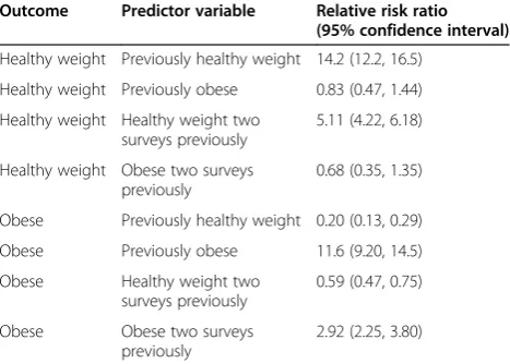
Table 2 shows estimated relative risk ratios and 95% confidence intervals obtained from the transition model. Pseudo R2for the model was 0.47 with 81% correct pre-dictions (compared to 59% correct prepre-dictions for an uninformative model) indicating moderate predictability of current BMI group for individuals based on BMI group at the two previous surveys. Predicted and observed tran-sitional probabilities showed only moderate agreement, al-though some of these categories included low numbers of participants (Additional file 2: Figure S1).
Table 1 Percentage changes in log likelihood
Variable at survey wave 5
Null model
Previous survey
Two surveys previous
Three surveys previous
Physical activity level −8062.1 −7703.1 −7648.9 −7601.2
4.5% +0.6% +0.6%
BMI group −8644.0 −4811.2 −4562.8 −4506.7
44.3% +2.9% +0.6%
Smoking status −10906.3 −2588.4 −2449.6 −2424.8
76.3% +1.2% +0.2%
Table 2 Relative risk ratios based on transitional model for BMI group (reference = overweight)
Outcome Predictor variable Relative risk ratio (95% confidence interval)
Healthy weight Previously healthy weight 14.2 (12.2, 16.5)
Healthy weight Previously obese 0.83 (0.47, 1.44)
Healthy weight Healthy weight two surveys previously
5.11 (4.22, 6.18)
Healthy weight Obese two surveys previously
0.68 (0.35, 1.35)
Obese Previously healthy weight 0.20 (0.13, 0.29)
Obese Previously obese 11.6 (9.20, 14.5)
Obese Healthy weight two surveys previously
0.59 (0.47, 0.75)
Obese Obese two surveys previously
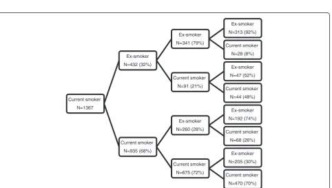
For smoking status, VIFs of between 6 and 24 indi-cated strong multicollinearity when more than one pre-vious survey was included as explanatory information in a transition model. However we were able to include an explanatory variable indicating whether or not a partici-pant was an ex-smoker two surveys previously as this did not result in multicollinearity and added useful pre-dictive information to the model. Figure 4 shows a prob-ability tree diagram for current smokers illustrating the additional predictive value of including being an ex-smoker two surveys previously as a predictor variable. In contrast, being a current smoker two surveys previously added little additional predictive value. Transitions from being an ex- or current smoker to never having smoked are not possible hence current smoker was chosen as the reference category and predictor coefficients indi-cating previous smoking status of never smokers were constrained to be (structurally) zero. Some participants reported never smoking after being classified as an ex-smoker or current ex-smoker at earlier surveys. These partici-pants were reclassified as ex-smokers. The transition model (shown below) included indicator variables for whether the participant was a current smoker in the previous sur-vey, an ex-smoker at the previous sursur-vey, or an ex-smoker at the previous two surveys.
logitπj¼β1jþI Exð Þ−1β2jþI Currentð Þ−1β3j
þI Exð Þ−1;−2β4j ð5Þ
where-1indicates status at the previous survey,-1,-2
indi-cates ex-smoker for both previous surveys.
Estimates obtained from the model showed that being an ex-smoker at the previous survey (but not being an ex-smoker two surveys previously) was associated with a doubling in relative risk of being an ex-smoker currently (RRR 2.01; 95% CI: 1.12, 3.63) whereas being an ex-smoker for both previous surveys was associated with a 12-fold increased relative risk of being an ex-smoker currently (RRR 12.8; 95% CI: 6.95, 23.5). Being a current smoker at the previous survey was associated with a 72% lower relative risk of being an ex-smoker currently (RRR 0.28; 95% CI: 0.16, 0.50). The final model had pseudo R2= 0.77 with 91% correct predictions (compared to 52% correct predictions for an uninformative model) hence smoking status for the previous surveys was highly predictive of current status for individuals. Predicted and observed transitional probabilities agreed to within 1% in all cases hence goodness-of-fit statistics indicated the model fitted the observed data well. Predicted probabilities showed previous never smokers had 99% (95% CI: 98.8%, 99.3%) chance of being a never smoker at the current sur-vey, 0.6% (95% CI: 0.4%, 0.8%) chance of being an ex-smoker and 0.3% (95% CI: 0.1%, 0.5%) chance of being a current smoker. Previous current smokers had 34% (95% CI: 32%, 37%) chance of being an ex-smoker in the current survey and 66% (95% CI: 63%, 68%) of being a current smoker. An ex-smoker for the two previous sur-veys had 4% (95% CI: 3%, 5%) chance of being a current
Current smoker
N=1367
Ex-smoker
N=432 (32%)
Ex-smoker
N=341 (79%)
Ex-smoker
N=313 (92%)
Current smoker
N=28 (8%)
Current smoker
N=91 (21%)
Ex-smoker
N=47 (52%)
Current smoker
N=44 (48%)
Current smoker
N=935 (68%)
Ex-smoker
N=260 (28%)
Ex-smoker
N=192 (74%)
Current smoker
N=68 (26%)
Current smoker
N=675 (72%)
Ex-smoker
N=205 (30%)
Current smoker
N=470 (70%)
smoker at the current survey and 96% (95% CI: 95%, 97%) chance of being an ex-smoker. However for ex-smokers at the previous survey, who were not ex-smokers two sur-veys previously, the transition probabilities were 21% (95% CI: 18%, 24%) for current smoking and 79% (95% CI: 76%, 82%) for ex-smoking.
Discussion
The plot we have illustrated visually depicts changes in categorical variables for individuals over time. However the marginal distribution at follow up time-points is not as clearly shown, therefore we recommend inclusion of a table above the stacked bars showing the marginal distri-bution at each time-point. Simple nominal logistic re-gression models can be used to formalise the visual information provided by the plot and estimate marginal and transitional probabilities as well as relative effects. Probability tree diagrams are useful in helping develop the models.
Transitional probabilities, in particular, provide useful and easily interpretable summary information. For ex-ample, based on ALSWH data, conditional on being overweight for two previous surveys, Australian women in their twenties had 23% (95% CI: 21%, 26%) probability of being obese at the next survey but only 7% (95% CI: 6%, 9%) probability of being of healthy weight (or under-weight). We suggest McFadden’s pseudo R2
as a sum-mary measure for assessing predictability of categorical outcomes and, to guide decisions on how many previous measures should be included in the transition models, we propose using variance inflation factors and percent-age increases in log likelihood.
Spaghetti plots are very useful for showing changes in a numerical variable for a limited number of individuals over time but are not applicable for categorical data or large numbers of individuals. Lasagne plots have been proposed as an alternative tospaghetti plots for categor-ical data and/or many individuals. There are however several other methods for graphically representing cat-egorical data but they have a number of limitations. For example, in the mosaic plot the relative frequency of each level of a variable and its relationship to another vari-able is represented by a mosaic of tiles [9]; see Additional file 3: Figure S2. A variable degree of shading for each tile is then incorporated to represent the degree of deviation from a null hypothesis of independence. However adding more variables increases complexity and showing the dis-tribution of a categorical variable over multiple waves of a longitudinal survey is not feasible.
Another technique is known as parallel sets [10]; a simi-lar concept to Sankey diagrams [11]. In these diagrams the relationship between variables is shown using parallelo-grams whose width is proportional to the frequencies involved (Additional file 4: Figure S3). Parallel sets are
appropriate for categorical data collected on large num-bers of participants over multiple surveys but the plot lacks simplicity and software to produce the figures is not readily available.
The lasagne plot we illustrate offers some advantages over these alternative methods in terms of ease of depic-tion and interpretadepic-tion. But, irrespective of which graph-ical method is used, the information obtained is only descriptive hence the need for methods that allow formal testing and estimation.
To simplify our illustration we restricted analysis to in-dividuals who provided complete responses over four surveys. However this restriction could be relaxed to in-clude all participants. In this case missing data could form an additional category and be included in the plot, tabulation and models. The addition of a missing data category could provide additional insights into the data. For example, it could show that certain categories in pre-vious surveys are associated with increased risk of missing data in subsequent surveys. It may also be of interest to tabulate the patterns of missing data across surveys. We illustrate the inclusion of missing data as a category in the graphical analysis of BMI categorised into healthy, over-weight/obese, or missing (Additional file 5: Figure S4). The plot suggests previous missingness predicts current missingness but missingness does not appear to be associ-ated with the other BMI categories of healthy weight and overweight/obese.
Conclusions
The lasagne plot we illustrate provides a simple way to show transitions in the status of individuals observed longitudinally. The regression models we suggest com-plement the plots and allow formal testing and reporting of marginal and transitional distributions. These analyt-ical tools can be implemented in standard statistanalyt-ical soft-ware such as SAS and Stata and can provide valuable insights into categorical variables measured on individuals at regular intervals over time.
Additional files
Additional file 1:SAS code for generating smoking status plot.
Additional file 2: Figure S1.Probability tree diagram for BMI group with observed and estimated transitional probabilities and 95% confidence intervals in brackets.
Additional file 3: Figure S2.Mosaic plot of smoking status at survey wave 1 compared to wave 2.
Additional file 4: Figure S3.Parallel sets diagram of smoking status transitions from survey waves 1 to 5.
Additional file 5: Figure S4.Plot and marginal distribution table of body mass index group with a missing category over survey wave for the Australian Longitudinal Survey of Women’s Health.
Additional file 6: Figure S5.Plot and marginal distribution table of smoking status over survey wave for ex-smokers at survey wave 2.
Additional file 7: Figure S6.Plot and marginal distribution table of smoking status over survey wave for current smokers at survey wave 2.
Abbreviations
ALSWH:Australian Longitudinal Study of Women’s Health; BMI: Body mass index; VIF: Variance inflation factor; RRR: Relative risk ratio.
Competing interest
The authors declare that they have no competing interest.
Authors’contribution
RH developed the plot methodology; MJ developed the modelling strategy and wrote the manuscript; GM and AD oversaw the project, provided supervision as well as critical input into the design and implementation; all authors reviewed and/or revised the manuscript and have approved it for submission.
Acknowledgements
Funding: The Australian Longitudinal Study on Women’s Health is funded by the Australian Department of Health. MJ and GDM are funded by the Australian National Health and Medical Research Council (APP1000986). RH is funded by the Australian Department of Health and AD is funded by the University of Queensland. The funding bodies had no role in the collection, analysis, and interpretation of data; the writing of the manuscript, or the decision to submit the manuscript for publication. There was no additional person who contributed materials essential for the study or who contributed to the preparation of this article.
Received: 18 November 2013 Accepted: 21 February 2014 Published: 27 February 2014
References
1. Hedeker D, Gibbons R:Longitudinal data analysis.Hoboken, New Jersey: John Wiley and Sons; 2006.
2. Swihart B, Caffo B, James B, Strand M, Schwartz B, Punjabi N:Lasagna plots: a saucy alternative to spaghetti plots.Epidemiology2010,21:621–625. 3. Wilkinson L, Friendly M:The history of the cluster heat map.Am Stat2009,
63:179–184.
4. Dobson AJ, Barnett A:An Introduction to Generalized Linear Models.3rd edition. Boca Raton, Florida: Chapman & Hall/CRC; 2008.
5. Lee C, Dobson AJ, Brown WJ, Bryson L, Byles J, Warner-Smith P, Young AF: Cohort profile: the Australian Longitudinal Study on Women's Health.
Int J Epidemiol2005,34:987–991.
6. Brown WJ, Trost SG:Life transitions and changing physical activity patterns in young women.Am J Prev Med2003,25:140–143.
7. Ware J, Lipsitz S, Speizer F:Issues in the analysis of repeated categorical outcomes.Stat Med1988,7:95–107.
8. Long J:Regression Models for Categorical and Limited Dependent Variables.
Thousand Oaks: Sage Publications; 1997.
9. Friendly M:Mosaic displays for multi-way contingency tables.J Am Stat Assoc1994,89:190–200.
10. Kosara R:Parallel sets: interactive exploration and visual analysis of categorical data.Trans on Visualization and Comput Graph2006,12:1–12. 11. Schmidt M:Der Einsatz von sankey-diagrammen im stoffstrommanagement.
Beitraege der Hochschule Pforzheim2006. Nr. 124.
doi:10.1186/1471-2288-14-32
Cite this article as:Joneset al.:Visualising and modelling changes in categorical variables in longitudinal studies.BMC Medical Research Methodology201414:32.
Submit your next manuscript to BioMed Central and take full advantage of:
• Convenient online submission
• Thorough peer review
• No space constraints or color figure charges
• Immediate publication on acceptance
• Inclusion in PubMed, CAS, Scopus and Google Scholar
• Research which is freely available for redistribution