R E S E A R C H
Open Access
A graphical method for practical and informative
identifiability analyses of physiological models:
A case study of insulin kinetics and sensitivity
Paul D Docherty
1*, J Geoffrey Chase
1, Thomas F Lotz
1and Thomas Desaive
2* Correspondence: paul. [email protected] 1Centre for Bioengineering, Department of Mechanical Engineering, University of Canterbury, New Zealand, Private Bag 4800, Christchurch, New Zealand
Full list of author information is available at the end of the article
Abstract
Background:Derivative based a-priori structural identifiability analyses of mathematical models can offer valuable insight into the identifiability of model parameters. However, these analyses are only capable of a binary confirmation of the mathematical distinction of parameters and a positive outcome can begin to lose relevance when measurement error is introduced. This article presents an integral based method that allows the observation of the identifiability of models with two-parameters in the presence of assay error.
Methods:The method measures the distinction of the integral formulations of the parameter coefficients at the proposed sampling times. It can thus predict the susceptibility of the parameters to the effects of measurement error. The method is testedin-silicowith Monte Carlo analyses of a number of insulin sensitivity test applications.
Results:The method successfully captured the analogous nature of identifiability observed in Monte Carlo analyses of a number of cases including protocol alterations, parameter changes and differences in participant behaviour. However, due to the numerical nature of the analyses, prediction was not perfect in all cases. Conclusions:Thus although the current method has valuable and significant
capabilities in terms of study or test protocol design, additional developments would further strengthen the predictive capability of the method. Finally, the method captures the experimental reality that sampling error and timing can negate assumed parameter identifiability and that identifiability is a continuous rather than discrete phenomenon.
1. Background
A number of physiological phenomenon have been modelled by formulating mathemati-cal representations of the relevant interactions. These models frequently incorporate variable parameters that can be identified to match the model representation to the observed behaviour. The value of these parameters is then used to characterise or quan-tify the response. However, with complex or large models, variable parameters can be selected that seem mathematically distinct, but in reality define the same observable effect and identification failure is certain. Thus, model identifiability analyses are used to test the selection of model parameters and ensure that they are mathematically distinct.
Approaches for the analysis of model identifiability typically assume continuous per-fect input data [1-3]. However, these derivative-based identifiability methods can
produce false assurances of identifiability. Recent dissatisfaction with the classical algo-rithms has resulted in the development of new methods that recognise assay error and discrete measurements as critical to identifiability [4,5]. The limitation of discrete data that is often subject of assay error often causes parameter trade-off [6-9] and thus lim-itation of the identified metrics clinical value. Thus, not only should a model be checked for identifiability in the classical a-priori sense, but the susceptibility of para-meters to mutual interference should also be tested.
For example, the Minimal Model of insulin sensitivity [10] has been shown to be identifiable using such methods [11-13]. However, with discrete data that is subject to assay error, parameter identification has sometimes failed [6,7,14]. Numerous Bayesian techniques have had success in limiting this failure [7,15-17], but they tend to force the parameters to diverge away from their true least square values, limiting the rele-vance of the model and exaggerating the influence of population trends on an indivi-dual test’s identified parameter values. Thus, widespread clinical application of these models has been limited by the ambiguity of results.
This article presents a novel graphical method for identifiability analysis that allows an identifiability analysis with consideration of noise and assay error. Furthermore, the method highlights areas for potential improvements to protocols and sampling times that would improve practical identifiability. At this stage of development, the method is limited to first-order, two-parameter models that allow a separation of parameters, but are typical of those found in pharmacokinetic (PK) and pharmacodynamic (PD) modelling.
2. Method and Study Design
The proposed method will be evaluated in-silicousing clinically validated models of insulin kinetics and the dynamic between insulin concentration and glucose decay. The method’s ability to predict the variation behaviour of identified parameters in a Monte Carlo analysis will be tested.
2.1 Proposed method process
To evaluate identifiability of a model, the integral formulations of the parameters are evaluated using an estimated test stimulus response. Thus, the method cannot be used in complete ignorance of the expected behaviour of the test participant. In particular, the approximate shape of the species concentrations as a result of the test protocol must be estimated, (this is a reasonable assumption in most PK/PD studies). The speci-fic steps are illustrated using a generalised function:
˙
X=f(X,Y,C,D,a,b) (i)
where: X is a measured species with a discrete resolution,Yis a species that is co-dependent withX and is not measureable,Cand Dare independent known input pro-files, andaandbare unknown model parameters
1. Rearrange governing equation to create a first order differential equation with separated parameters in terms of a-priori, constant and measurable concentration terms
˙
2. Derive the integral formulation of this governing equation
Xi−X0=a
i
0
f1(X,Y,C)dt+b
i
0
f2(X,Y,C)dt+
i
0
Ddt (iii)
where:iis each measured sample time after the first.
3. Evaluate the integral of the coefficients of each parameter between 0 and each proposed sample time using an assumed participant response to the test stimulus.
˜ a=
i
0
f1(X,Y,C) b˜=
i
0
f2(X,Y,C) (iv)
4. Divide the resulting values by their respective means to normalise the coeffi-cients.
a=a˜/a¯˜ b=b˜/¯˜b (v)
5. Subtract one set of coefficients from the other and define the 2-norm of the result (||Δ||2).
||||2=||a−
b||2 (vi)
6. Any distinction at all between the coefficients would imply identifiability (i.e. if || Δ||2 ≠0). In reality, the effect of assay error on parameter identification is inversely proportional to the magnitude of this distinction (and proportional to the magni-tude of any assay error (ε)):
Variability=μ ε
||||2 (1)
where:μis a proportionality factor that incorporates factors such as the relative con-tribution of the parameter to the derivative of the relevant species concentration in the governing differential equation, and the absolute magnitude of the noise at the sampled times in relation to the relative magnitude of the parameter coefficient.
Thus, the method cannot accurately predict the coefficient of variation that a Monte Carlo analysis may find. However, it can predict the change of variation that might be observed when changes are made to the test sampling or stimulus protocols.
2.2 The dynamic insulin sensitivity and secretion test (DISST) model 2.2.1 Insulin pharmacokinetics
Initially, a validated model of insulin PKs [18,19] is used to evaluate the method described, and is defined:
˙
I=−nkI−nL I
1 +αII− nI VP
(I−Q) +xLUN+ UX
VP
(2)
˙ Q= nI
VQ
(I−Q)−nCQ (3)
The model is used in the dynamic insulin sensitivity and secretion test (DISST) to define the PKs of insulin due to test stimulus [18,20]. The model assumes that plasma insulin (I) is sampled. A traditional derivative based identifiability analysis of the model presented in Equations 2 and 3 using Ritt’s pseudo-division algorithm [1,21] is pre-sented in Appendix 1.
2.2.2 Pharmaco-dynamics of glucose and insulin
The parameters of the glucose-insulin PDs can also offer insight into the identifiability of parameters. The DISST model of glucose-insulin PDs is defined [18,19]:
˙
G=−pG(G−Gb)−SI(GQ−GbQb) + PX VG
(4)
where: equation nomenclature is defined in Table 2.
Although the structural identifiability of Equation 4 is trivial it is also presented in Appendix 1.
2.3 Participants
Parameter values from two participants of the pilot investigation of the DISST [18] are used to generate in-silico simulated data to construct and demonstrate the method proposed here. In-silicodata is used in this analysis because it allows protocols to be changed to illustrate the impact on identifiability. The participant characteristics that are summarised in Table 3 represent the extremities of the range of cases encountered in typical research studies of insulin sensitivity.
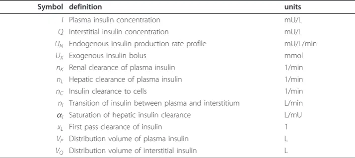
Table 1 Nomenclature from Equations 2 and 3
Symbol definition units
I Plasma insulin concentration mU/L
Q Interstitial insulin concentration mU/L
UN Endogenous insulin production rate profile mU/L/min
UX Exogenous insulin bolus mmol
nK Renal clearance of plasma insulin 1/min
nL Hepatic clearance of plasma insulin 1/min
nC Insulin clearance to cells 1/min
nI Transition of insulin between plasma and interstitium L/min
aI Saturation of hepatic insulin clearance L/mU
xL First pass clearance of insulin 1
VP Distribution volume of plasma insulin L
VQ Distribution volume of interstitial insulin L
Table 2 Nomenclature from Equation 4
Symbol definition units
G Glucose concentration mmol/L
Q Interstitial insulin concentration mU/L
Gb Basal glucose concentration mmol/L
Qb Basal interstitial insulin concentration mU/L
pG Glucose dependant glucose clearance 1/min
SI Insulin sensitivity L/mU/min
PX Exogenous glucose bolus mmol
2.4 Simulated test protocol
The simulated protocol is similar to the DISST test; a 10 g glucose bolus is adminis-tered at t= 7.5 and a 1 U insulin bolus at t = 17.5. The test duration is 60 minutes with a 5 minute sampling frequency. The UNprofile is defined as a step function with three stages including basal, first and second phase production rates. The first phase of insulin production has a five-minute duration and begins with the glucose bolus. Simu-lations of plasma and interstitial insulin are completed using Equations 2 and 3, the parameter estimation equations from [22], nLand xL values from Table 3 and an aI
value of 0.001 L/mU. Glucose is simulated using Equation 4 and the interstitial insulin profile obtained in the evaluation of Equations 2 and 3.
2.5 Iterative integral method
The analyses of this study will use the iterative integral method to identify parameters [20,23]. Although the method has been presented [20], it is repeated in brief in Steps 1-5 below:
1. The method converts the model governing equations to their integral formulation.
2. The parameter coefficients and the remainder terms are evaluated betweent= 0 and the sample times.
3. The coefficients form the LHS of a matrix equation in terms of the parameters, while the remainder terms form the RHS. This matrix is evaluated to get parameter values.
4. These parameter values are used to update the coefficient evaluations in step 2, which enables a more accurate matrix equation in step 3.
5. Step 4 is iterated until convergence is achieved.
2.6 Analysis
A series of parameter and sampling scenarios were analysed using the models pre-sented in a Monte Carlo analysis. Clinically measured physiological parameters of the NGT participant presented in Table 3 were used to define simulated responses to the test protocol described in Section 2.4. Samples were obtained from the simulated pro-files at the defined times. Each iteration of the Monte Carlo analysis adds normally dis-tributed assay error (the error magnitude is defined within each section). 100 iterations are used for each analysis with parameter identification by the iterative integral method. Only simulated profiles from the NGT participant are used until Section 3.2.2. Each scenario will present the mean value of those identified in the Monte Carlo Table 3 Anatomical and identified parameter values
Glucose tolerance Sex Age BMI UN† I clearance VG SI
Ub U1 U2 nL xL
NGT M 22 21.5 26.6 487.7 9.7 0.218 0.797 9.75 20.95
IGT* F 57 33.9 115.5 233.6 150.7 0.064 0.822 13.35 2.236
Anatomical and identified parameter values (using the iterative integral method) of normal-glucose tolerant (NGT) and impaired glucose tolerant (IGT) participants of the DISST pilot investigation. (* The IGT participant had suspected, yet un-diagnosed, type 2 diabetes at the time of testing,†Ub, U1andU2represent the basal, first and second phases of insulin
simulation normalised by the simulation value from Table 3, and the coefficient of var-iation (CV) of each identified parameter (i.e. A mean of 1 and standard devvar-iation of 0 implies perfect identification). The CV values are the paramount indicator of para-meter trade-off during identification. The CV values are thus was compared to the ε/|| Δ||2 value defined using the methods of Section 2.1 to obtained values forμthat line-arise Equation 1.
2.7 Cases tested
A series of indicative cases will be investigated to show how the selection of model parameters, sample placement, participant behaviour and protocol dosing can have an effect on model identifiability.
•The insulin pharmacodynamic model will include five variable parameters to be identified to confirm the robustness and convexity of the iterative integral method, and to confirm the findings of the traditional derivative-based identifiability analysis.
•Parameter interference ofnLand nKwill be analysed. The nature of identifiability will be explored by alteration of theaIterm that moderates the denominator of nL
in Equation 2.
•The effect of sample selection on parameter identification of nTand VPwill be measured. (nTis the addition of nLand nK).
•The effects of sample omissions onSIandVGidentification are measured. •The disparity of parameter identifiability in insulin resistant and sensitive indivi-duals will be assessed usingpGandSIas variable model parameters.
•The protocol proposed in Section 2.4 will be altered to see if the identifiability of insulin resistant participants can be improved.
•Measured samples that the proposed method claims are not valuable to stable identification are ignored and the identification process is repeated to confirm the prediction.
All cases will be tested with 1% and 3.5% normally distributed noise added to the vir-tually obtained data (to a maximum of 3 standard deviations).
3. Results
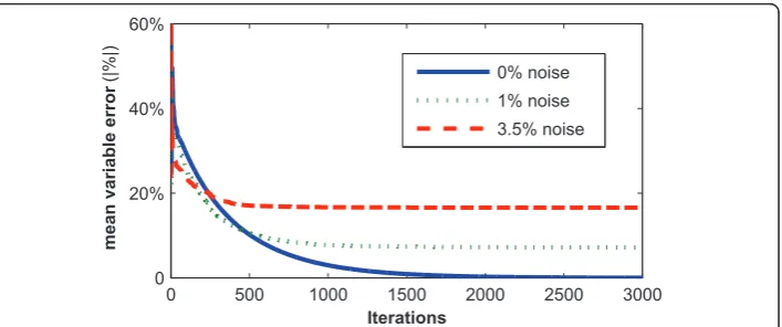
3.1 Analysis of the insulin pharmacokinetic model 3.1.1 Confirmation of global model identifiability
When the sampled data is used in the iterative integral method to define nL,nK,nI/VP,
3.1.2 Hepatic and renal clearance rate identification
To understand why the addition of noise disables the identification, the case of inter-ference betweennKand nLis tested. In this analysis, all parameters of Equations 2 and 3 are set as constants and onlynL andnK are identified as parameters. From the ana-lyses in Appendix 1 and Section 3.1.1, parameter convergence is assured for the noise-less case. However, for the 1% and 3.5% noise cases parameter interference causes considerable parameter divergence in the value of the identified parameters compared to the actual values usedin-silico. The Monte Carlo analysis described in Section 2.6 is used to evaluate these parameters in the presence of noise and the results are shown in Table 4.
The matrix equation used by the iterative integral method is a re-arrangement of Equation 2 and is in the form:
−nk
i
0
Idt−nL
i
0
I
1 +αII dt
=Ii−I0+
nI Vp
i
0
(I−Q)dt−xL
i
0
UNdt+
i
0
UX Vpdt
(2a)
where:i= 5, 10, 15, ..., 60 minutes, matching sampling times.
Thus, the value of the ||Δ||2 term can be obtained for this model and sampling pro-tocol as:
||||2=
⎛ ⎜ ⎝ i 0Idt 1 n i 0Idt ⎞ ⎟ ⎠− ⎛ ⎜ ⎜ ⎝ i 0 I
1 +αII dt 1 n i 0 I
1 +αII dt ⎞ ⎟ ⎟ ⎠ 2 = 0.032
0 500 1000 1500 2000 2500 3000
0 20% 40% 60%
Iterations
mean variable error
(|%|) 0% noise
1% noise 3.5% noise
Figure 1Convergence of 5 parameter case. Mean absolute percentage error between the simulation and identified parameters in the presence of 0%, 1% and 3.5% random assay error, with respect to iterations of the iterative integral identification approach.
Table 4 Variation in identifiednKandnLvalues
Noise 0% 1% 3.5%
Saturation aI= 0.001 aI= 0.05 aI= 0.001 aI= 0.05 aI= 0.001 aI= 0.05
nK 1(0) 1(0) 0.952(0.297) 0.999(0.017) 0.946(0.836) 1.004(0.059)
nL 1(0) 1(0) 1.035(0.214) 1.001(0.008) 1.041(0.595) 1.000(0.028)
The normalised parameter variation (mean(CV)) whennKandnLare identified model parameters with distinct simulated
However, Table 4 shows that ifaIis increased significantly to 0.05 L/mU, an arbitrarily chosen value that is not necessarily representative of physiology [24], parameter conver-gence is more stable. The ||Δ||2term can be re-identified with the exaggeratedaIvalue.
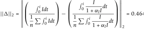
||||2=
⎛ ⎜ ⎝ i 0Idt 1 n i 0Idt ⎞ ⎟ ⎠− ⎛ ⎜ ⎜ ⎝ i 0 I
1 +αII dt 1 n i 0 I
1 +αII dt ⎞ ⎟ ⎟ ⎠ 2 = 0.464
Thus, the parameters identified with the exaggerated aIterm should have approxi-mately 15 times smaller variability than those identified with the accepted aIvalue. Table 4 shows the effect of the aIdistinction on the identified parameter values.
Table 4 shows the distinction between the effects of noise on identified parameters when theaIterm is changed. Although the 0% noise case indicates that the parameters are uniquely identifiable, at 1% noise the variation in the identified values limits their clinical viability. At 3.5% noise, which may be expected in a real clinical setting, the parameters are no longer uniquely identifiable. This is illustrated by the very large CVs of the parameters. However, when the aIterm is significantly increased, unique
iden-tifiability is once again possible, even with 3.5% noise. The mean ratio of variation caused by the disparateaIvalues was approximately 1:20. This is larger than the ratio predicted by the method (1:15), but still represents a positive outcome in terms of pre-dicting the relative magnitude of the change.
The reason for this outcome can be observed in the increased contrast between integral formulations of the parameter coefficients. The contrast is shown graphically in Figure 2.
The difference between the curves at the sample times indicates the identifiability of the model parameters in this two-parameter case. Thus, when the saturation term is increased, the coefficients of the parameters are more distinct and identifiability is increased. Despite the positive findings of the typical identifiability analysis, a
0 10 20 30 40 50 60
0 0.2 0.4 0.6 0.8 1 1.2 1.4 1.6
||Δ||2=0.032
Time [mins]
0 10 20 30 40 50 60
0 0.2 0.4 0.6 0.8 1 1.2 1.4 1.6 1.8 2
||Δ||2=0.464
Time [mins]
nL coeff.
nK coeff. Samples
Figure 2Renal and hepatic clearance coefficient integrals. The distinctions between the integral form of the hepatic and renal clearance coefficients when the standard (left) and exaggerated (right)aIvalues
saturation value of 0.001 L/mU causesnKand nLto become uniquely un-identifiable in a real clinical setting. This outcome may be considered as an elementary finding that should be inferred with a quick observation of Equation 2. However, it points to a fail-ing of typical a-priori identifiability tests that this approach can negate with a quick graphical analysis.
The findings of this analysis also show that the functional effects of nLandnKon insulin concentration in Equation 2 are so similar that there would be a negligible effect if the terms are combined. As such, further analysis of this model will use a combined nLandnK term (nT) without the saturation term, which is negligible except at extremely high insulin concentrations. Equation 2 is thus redefined in Equation 5:
˙
I=−nTI− nI VP
(I−Q) +xLUN+ UX VP
(5)
3.1.3 Plasma insulin distribution volume and insulin clearance identifiability
To identifynTandVp the form of the governing matrix equation is:
VP
i
0
(nI(Q−I) +UX)dt−nT
i
0
Idt=Ii−I0−xL
i
0
UNdt (5a)
where:VP= 1/Vp
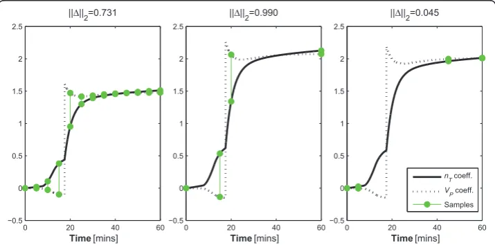
As with thenKandnLanalysis, the 0% noise case exactly reproduced the simulation values. Figure 3 shows the coefficients of the two parameters and three sampling pro-tocols. In this case, Protocol 1 uses the 5 minutely sampling defined in Section 2.4. However, Protocol 2 uses samples at t= 0, 15, 20, and 60, and Protocol 3 uses samples at t= 0, 5, 45, and 60 minutes. Thus, Protocol 1 requires 13 samples while both proto-col 2 and 3 only require four samples.
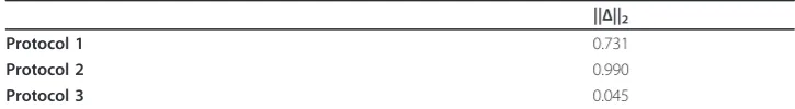
The ||Δ||2 terms can be defined for each of these protocols (Table 5) and the coeffi-cients are displayed graphically in Figure 3.
The ||Δ||2values indicate that Protocol 3 will be comparatively unable to reproduce the simulation values. Contrary to the expected result that parameter identification is
0 20 40 60
−0.5 0 0.5 1 1.5 2 2.5
||Δ||2=0.731
Time [mins]
0 20 40 60
−0.5 0 0.5 1 1.5 2 2.5
||Δ||2=0.990
Time [mins]
0 20 40 60
−0.5 0 0.5 1 1.5 2 2.5
||Δ||2=0.045
Time [mins]
nT coeff. VP coeff. Samples
best with frequently sampled Protocol 1, the method predicts that the sparsely sampled Protocol 2 will be slightly more accurate.
Table 6 shows the parameter convergence and variability for the exact same model with the three different sampling protocols.
It is evident that although Protocols 2 and 3 contain the same number of samples, the resolution of the identified parameters is considerably reduced in Protocol 3. In effect, Vpwas un-identifiable with Protocol 3. This result occurs because of the lack of distinction in the coefficients of the parameters at the sample times as indicated in Table 5 and Figure 3.
Thus, the method predicted the poor performance of the third protocol while it pre-dicted much lower variability for both Protocols 1 and 2. However, it also suggests that Protocol 2 would improve slightly upon Protocol 1, which was not the case as both protocols performed equally in terms of parameter identifiability. It is expected that it’s equality of variance is an artefact of the normalisation as a function of mean coefficient at the sample value, artificially lowering the magnitude of the ||Δ||2 terms in Protocol 1.
Overall, these findings highlight the inefficiency, extreme clinical burden and inten-sity of frequent sampling in contrast to well-positioned and infrequent sample timing. More specifically, Protocol 1 used 9 more samples than Protocol 2 with significant added clinical intensity and assay cost (~200% more!) for absolutely no information gain. This outcome was successfully predicted by the identifiability analysis method presented.
3.2 Analysis of the glucose PD model
Equation 4 will be used in the analysis of identifiability of terms frequently used to model the PDs of insulin and glucose. All analyses in this section will simulate insulin concentration profiles for the plasma and interstitium only once for each Monte Carlo analysis. Thus for clarity and simplicity, it is assumed that insulin is not subject to assay error here. Furthermore, while glucose assay error from a blood gas analyser is approximately 2%, errors of 1% and 3.5% will be used for consistency with Section 3.1. As such, the resultant coefficients of variation should not be considered fully applicable clinically, but merely as an indication of parameter trade-off during identification. The Monte Carlo analysis method with the NGT participant described in Section 2.3 is
Table 5 ||Δ||2values from three sampling protocols defined in Section 3.1.3
||Δ||2
Protocol 1 0.731
Protocol 2 0.990
Protocol 3 0.045
Table 6 Protocol dependence of identifiednTandVPvalues
Noise 1% 3.5%
Protocol 1 2 3 1 2 3
nT 1(0.004) 1(0.003) 0.973(0.012) 1.003(0.012) 1.001(0.014) 0.958(0.045) VP 1.001(0.014) 0.995(0.012) 1.231(0.175) 0.999(0.047) 0.995(0.051) 1.190(0.463)
repeated for the glucose PD model. The IGT participant will be used in tandem with the NGT participant from Section 3.2.2.
3.2.1 Insulin sensitivity and distribution volume
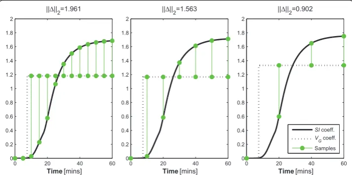
Use of the DISST model typically entails the identification of SIandVGin Equation 4 [18,20,25]. As such, this case is tested using the proposed method and three potential sampling protocols. Specifically, Protocol 1 uses the 5-minute sampling resolution described in Section 2.4, while Protocols 2 and 3 use 10 and 20-minute resolutions, respectively. Figure 4 and Table 7 indicate that these parameters are uniquely identifi-able in the presence of measurement noise given a surprisingly small number of data points.
Table 7 shows that parameter stability is generally very high even in a sparsely sampled data set with a relatively high level of noise. This result was expected due to the relatively large difference in the coefficient integrals shown in Figure 4 for each of the sampling protocols. Thus, like the case ofVPand nT, intelligent sample timing can significantly reduce clinical burden and study cost with negligible loss of information. Furthermore, the proposed method successfully predicted this outcome.
3.2.2 Insulin sensitivity and glucose dependent decay
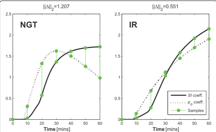
Model-based studies of insulin sensitivity frequently identify a parameter synonymous withpGin addition toSIandVGas parameters when using the Minimal Model [10] or similar. However, although these parameters are mathematically distinct, they are known to trade-off during identification and practical identifiability is not generally assured. It has been reported that these issues can be exacerbated for insulin resistant (IR) individuals [7,8]. Thus, the second, IGT participant defined in Table 3 will also be analysed.
Some insight into the parameter trade-off during identification of dynamic test data can be seen in Figure 5 that contrasts the integral formulations of the parameter coeffi-cients based on glucose tolerance status. The contrasting shape of the integral formula-tions of the parameter coefficients is best observed in the pG coefficient. The pG coefficient is the only term in Equation 4 that could possibly become negative. Thus, the integral of the coefficient can form a convex shape that contrasts well with the
0 20 40 60
0 0.2 0.4 0.6 0.8 1 1.2 1.4 1.6 1.8 2
||Δ||2=1.961
Time [mins]
0 20 40 60
0 0.2 0.4 0.6 0.8 1 1.2 1.4 1.6 1.8 2
||Δ||2=1.563
Time [mins]
0 20 40 60
0 0.2 0.4 0.6 0.8 1 1.2 1.4 1.6 1.8 2
||Δ||2=0.902
Time [mins]
SI coeff. VG coeff. Samples
coefficient of SI as seen for the NGT participant in Figure 5. However, the negative coefficient of pGcan only occur when the participant’s glucose concentration goes below the basal concentration. Thus, as only NGT participants achieve such concentra-tion reducconcentra-tions in typical dynamic insulin sensitivity tests, the parameter identifiability of IR participants is impaired in comparison. In particular, Figure 5 (right) shows mini-mal difference and a much smini-maller ||Δ||2 value for this IR individual indicating increas-ing potential for parameter trade-off in the identification process and loss of effective identifiability. This is despite an identical test protocol and model.
As mentioned, this limitation of the Minimal Model has been reported, but not explained in the literature until now.
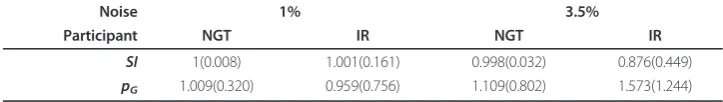
Table 8 shows the parameter error when the 60 minute 10-minute sampling protocol is used.
It is apparent that the insulin resistant individual’s parameter identifiability is much lower than the NGT participant despite the identical PD model, test protocol and identification process. Table 8 highlights this result, as well as the increasing loss of identifiability as assay error increases. This is in accordance to published findings and the proposed method’s prediction.
3.2.3 A hypothetical protocol to enable pGidentification in dynamic tests
To forcibly remove this ambiguity introduced by the comparable coefficients of the IR individual, the protocol of the DISST could be altered. After an initial observation of
Table 7 Sample resolution dependence of identifiedSIandVGvalues
Noise 1% 3.5%
Protocol 1 2 3 1 2 3
SI 1.001(0.007) 1.002(0.008) 1(0.016) 1.002(0.028) 1.002(0.033) 1.010(0.054)
VG 1(0.012) 1(0.014) 1.001(0.029) 0.998(0.046) 1.001(0.049) 0.990(0.087)
The normalised mean and (CV) of the glucose PD parameter values from the three proposed sampling resolutions.
0 10 20 30 40 50 60
0 0.5 1 1.5 2 2.5
||Δ||2=1.207
Time [mins]
NGT
0 10 20 30 40 50 60
0 0.5 1 1.5 2 2.5
||Δ||2=0.551
Time [mins]
IR
SI coeff.
p
G coeff.
Samples
the effect of the insulin bolus on glucose concentration, more insulin could be intro-duced to ensure that the participant’s glucose concentration is maintained approxi-mately 0.5 mmol/L below the basal concentration. Such a protocol may include an extension of the protocol described in Section 2.4 wherein a period of slight hypogly-caemia is achieved for each participant with a series of participant-specific insulin boluses administered with feed-back control.
To allow a fair comparison between the variability of the parameters of the proposed protocol and the protocol used in Section 3.2.2 the sampling regimen and test duration will be maintained. Thus, the additional insulin is administered as a bolus t= 32.5 minutes. In a clinical setting, the magnitude of the bolus would be participant-specific and dependent on the glucose concentration response alone (as glucose can be assayed in real-time). Note that this task would be very difficult and potentially dangerous in a regular clinical setting. In particular, the amount of insulin required would vary between participants, and must be estimated in ignorance of endogenous insulin pro-duction. This may cause a high incidence of potentially harmful hypoglycaemia. This protocol is only mooted to illustrate the ability of the method, and in reality the intro-duction of additional insulin could be applied slowly and safety would be assured.
For the case of the IR participant presented here, reducing glucose sufficiently would require a 3U bolus att= 32.5 minutes.
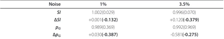
The proposed protocol would alter the shapes of the integral of the parameter coeffi-cients for the resistant individual. In doing so, it is hypothesised that it would increase the distinction between these curves to avoid the similarity seen in Figure 5 (right) to ensure identifiability. The ||Δ||2value obtained for the IGT participant and the updated protocol indicates a reduction in variability ratio of approximately 1:2.2. Figure 6 contrasts with Figure 5 (right) as it shows how the added bolus significantly increases the distinction between the coefficients of the identified parameters. Table 9 shows the outcomes of this analysis.
Although the inhibitive CV values for the parameters indicate that the proposed pro-tocol could not be used clinically, the variability decreased in the order predicted by the identifiability method presented. The hypothetical protocol presented has con-firmed the reasons discussed for the poor parameter identification observed in many clinical studies which utilise these two competing parameters [7,8]. Furthermore, it demonstrates a limitation of traditional identifiability methods, which provide an eva-luation of identifiability in ignorance of probable participant behaviour or test protocol design.
The protocol presented would be virtually impossible to apply clinically in the 60 minute duration as it is shown here. However, this analysis was limited by the need for a comparable duration and sampling regimen to Section 3.2.2. The method could thus be used to define similar protocols that could yield data that enables unique identifica-tion of these parameters. If such protocols are pursued, they would most likely require
Table 8 Participant dependence of identifiedSIandpGvalues
Noise 1% 3.5%
Participant NGT IR NGT IR
SI 1(0.008) 1.001(0.161) 0.998(0.032) 0.876(0.449)
pG 1.009(0.320) 0.959(0.756) 1.109(0.802) 1.573(1.244)
two sections in a much longer test. The first section would involve the protocol defined in Section 2.4, and would be followed immediately by an infusion of insulin designed to safely bring the participant’s glucose concentration to 0.5 mmol/L below the basal level. Robust results would be most assured if the participant’s glucose con-centration was maintained below this level for approximately 30 minutes, and thus, the protocol would most likely require about 2 hours. However, a stable result both in terms of SIandpGwould be generally assured.
3.2.4 Removal of redundant points
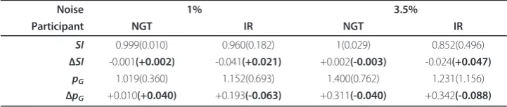
The t= 40 minute sample in Figure 5 (left) and t= 30 in Figure 5 (right) show vir-tually no distinction between the coefficients of either profile. Thus, according to the theory presented, it should provide no value to the identification process. To test this, the analysis of Section 3.2.2 is repeated with these samples removed. Figure 7 shows how the omitted data point do not significantly alter the distinction shown in Figure 5 (Section 3.2.2). Table 10 shows how the identified parameters were affected by the omission of data that the method implied were redundant.
0 10 20 30 40 50 60
0 0.5 1 1.5 2 2.5 3
||Δ||2=1.237
Time [mins] SI coeff.
pG coeff.
Samples
Figure 6Effect of an alternative protocol to maximise parameter distinction in IR individuals. The effect of the added insulin bolus on the distinction of the coefficient integrals ofpGandSIfor the IR
participant.
Table 9 Effect of the added insulin bolus on the identifiability ofSIandpGfrom the IR
participant
Noise 1% 3.5%
SI 1.002(0.029) 0.996(0.070)
ΔSI +0.001(-0.132) +0.120(-0.379)
pG 0.989(0.369) 0.992(0.969)
ΔpG +0.030(-0.387) -0.581(-0.275)
Parameter convergence from the proposed hypothetical protocol.ΔSIandΔpGshow the change between these values
The findings of this analysis imply that the omission of the samples that were assumed to be obsolete had little effect on the outcome of the identification process. Most changes were very small and only those for the particularly un-stable parameters showed any significant changes.
3.3 The value ofμ
The value ofμin Equation 1 can be used to enable prediction of the probable variabil-ity in the identified parameters in a Monte Carlo simulation. Thus, the effects of proto-col changes on the parameter identifiability can be predicted without the need for numerous Monte Carlo simulations. To identify the value of μ linear relationships between the CV values obtained and the ε/||Δ||2values are defined. As noiseless iden-tifiability of all models has been proven, the y-intercept can be assumed at zero, and μcan be identified using Equation 6:
μ= 1
N
CV
(ε/||||2)
(6)
Figure 8 shows the adherence ofμto linear relationships while Table 11 shows the value of μfor the different parameters.
0 10 20 30 40 50 60
0 0.5 1 1.5 2 2.5
||Δ||2=0.528
Time [mins]
0 10 20 30 40 50 60
0 0.5 1 1.5 2 2.5
||Δ||2=1.336
Time [mins]
SI coeff.
pG coeff.
Samples
Figure 7Effect of omitting assumed negligible samples. The coefficient comparison in alternative sampling protocols that omit the samples that according to Figure 5 have almost negligible value in terms of identifiability due to the very small magnitude of distinction at the sample times.
Table 10 The effect of targeted sample omission
Noise 1% 3.5%
Participant NGT IR NGT IR
SI 0.999(0.010) 0.960(0.182) 1(0.029) 0.852(0.496)
ΔSI -0.001(+0.002) -0.041(+0.021) +0.002(-0.003) -0.024(+0.047)
pG 1.019(0.360) 1.152(0.693) 1.400(0.762) 1.231(1.156)
ΔpG +0.010(+0.040) +0.193(-0.063) +0.311(-0.040) +0.342(-0.088)
Parameter normalised mean and (CV) values of identified parameters with the omission of the assumed negligible data points.ΔSIandΔpGare the change in values between this analysis and Section 3.2.2. The boldΔCV values are the key
Table 11 presents the μvalues identified by the gradients of the regression lines It can be observed that no single value for μcan be applied across all models and that different parameters are considerably more susceptible to the distinction of the parameter coefficients. However, the general adherence to the linear relationships observed in most examples implies that the form of Equation 1 is accurate for this purpose with the possible exception of SIin Sections 3.2.2 and 3.2.4.
0 0.75 1.5
50% 100%
ε/||Δ||2
CV(%)
Section 3.1.2
μ (nL)
μ (nK)
0 0.5 1
25% 50%
ε/||Δ||2
CV(%)
Section 3.1.3
μ (nT)
μ (V P)
0 0.025 0.05
5% 10%
ε/||Δ||2
CV(%)
Section 3.2.1
μ (SI)
μ (V G)
0 0.05 0.1
75% 150%
ε/||Δ||2
CV(%)
Section 3.2.2−3.2.4
μ (SI)
μ (p G)
Figure 8Linear regression ofμ. Comparisons between CV values andε/||Δ||2terms to provide parameter specific values forμ.
Table 11μvalues from the various analyses
Analysis Parameter μ
Section 3.1.2 nL 0.560
nK 0.801
Section 3.1.3 nT 0.081
VP 0.683
Section 3.2.1 SI 1.48
VG 2.41
Sections 3.2.2 and 3.2.4 SI 6.45
4. Conclusions
The method presented was able to predict and explain the parameter identifiability behaviour exhibited in models of insulin kinetics and insulin/glucose dynamics. This capability is in direct contrast to the traditional derivative-based identifiability analysis [1,3,11-13] that can only provide a confirmation of an infinitesimal distinction of the parameters in the governing equations. In addition to the ability to predict parameter identifiability, the method has been shown to be able to aid sample selection and explain the non-identifiability of thepGterm in common insulin sensitivity tests for IR participants of dynamic tests. It was also used to derive and justify a novel protocol to make this parameter more identifiable in this subgroup. Furthermore, the method also accurately predicted sample redundancy.
Like the proposed method, the method proposed by Raue et al. [4] recognises the ability of apparently identifiable parameters to become practically non-identifiable in the presence of assay error and discrete sampling. The Raue et al. method requires numerous simulations and parameter identification processes to characterise the model sensitivity to variations in each model parameter. In contrast, the proposed method allows a quick graphical analysis, which can produce immediately apparent and intui-tive results. Furthermore, the proposed method can quickly appraise protocol variants, and provide indications of the reason for practical non-identifiability. The method of Raue et al. is a more general method as it can appraise most model configurations, whereas the proposed method is currently limited to models with two separable parameters.
In reality, many models utilise more than two parameters to describe physiological kinetics and seek to identify all at once. It is expected that development of the pro-posed method will enable identifiability analyses of such models. However, more care must be taken to construct the coefficient integral formulations as combinations of parameters that may come into conflict. This task would require the contrast between the most deleterious combinations of integral coefficients to be measured. However, this point was not explored in this study, as the goal was to introduce the overall approach.
Only cases with separable parameters in terms of measured species were analysed. In reality, some model parameters are intrinsically linked and this method will not work. An example of linked parameters would be insulin sensitivity and insulin effect satura-tion that requires a Michaelis-Menten formulasatura-tion. In addisatura-tion, some parameters effect remote, un-measured concentrations or masses and are thus not able to be identified with this method. For example, the nC term in Equation 3 could not be evaluated for identifiability using this method without the inclusion of measurements of interstitial insulin [26]. As such, this method should not replace the traditional identifiability ana-lysis, but be used in tandem with it (or methods such as Raue et al.[4] or similar) to produce both theoretical and practical investigations of identifiability.
search, and likely test outcomes could be cases that can be safely evaluated prior to clinical testing.
There is also an assumption that the model captures all of the dynamics of the sys-tem perfectly. In reality no model can provide such accuracy. In particular, Figures 4, 5, 6, 7 show a sample taken att= 10 for glucose. In reality, this sample will be affected heavily by error caused by incomplete mixing, and although the method presented indicates that this is a valuable sample, if it is used in the glucose pharmacodynamic model of Equation 5, the resultant parameters will be overly influenced by an un-mod-elled mixing effect.
Although the method has limitations and potential for improvement, it can provide valuable information at a study design stage, as well as valuable identifiability informa-tion not available from typical methods. It can differentiate between the applicability of different dynamic tests based on cohorts, and also help to define optimal sample tim-ing and frequency. In particular, it explained the observation of poor parameter con-vergence in the Minimal Model for insulin resistant participants that has been widely reported but without clearly defining the cause. Thus, despite the method’s limitations, it should still be used in the design stage of a study to ensure that the resultant clinical data can provide usable results, and time and money is not wasted.
Finally, the method has highlighted the limitation of discrete binary identifiability analyses as providing potentially misleading assurances of parameter identifiability in real clinical applications, and shown that identifiability is instead a continuous artefact of sample timing and the distinction between parameter coefficients.
Appendix 1: Structural identifiability
A1.1 Structural identifiability of the insulin model
Using the method of algebraic derivative approach of [21] and refined in [1] the iden-tifiability of the model can be confirmed. Using the ranking:
[UN <UX<U˙N <U˙X<Y<Y˙ <Y¨ <I<Q<˙I<Q˙]
generates the characteristic set of Equations 2 and 3.
− n2I VPVQ
Y+
nC+
nI VQ
˙
Y+nKY+nL Y
1 +αY + nI VP
Y+UX
VP
+xL(UN)
. . .
. . .+Y¨+nKY˙+nL ˙ Y
1 +αY˙ + nI VP ˙ Y+U˙X
VP
+xL(U˙N)
(3a)
˙
Y+nKY+nL Y
1 +αY + nI VP
(Y−Q) +UX
VP
+xL(UN) (2b)
if: Y=I
Thus, the following coefficients can be defined:
˙
Y : (nC+nK+ nI VP
+ nI
VQ
) Y:
nK+
nI VP
nC+ nI VQ
− n2I
VPVQ
˙ Y
1 +αY˙ :nL
Y
1 +αY :nL(nC+ nI VQ
˙ UX :
1
VP
UX: 1
VP (nC+
nI VQ
)
˙
UN :xL UN:xL(nC+ nI VQ
)
Using arbitrary values for the coefficients confirms global identifiability of the insulin kinetic model of Equations 2 and 3.
A1.2 Structural identifiability of the glucose model
The structural identifiability of the glucose model is considerably less complex than the insulin kinetic model. In particular, the characteristic set is defined:
˙
G+pG(G−Gb) +SI(GQ−GbQb)−VPXG (4a)
and thus the coefficients are defined:
G:pG GQ:SI
PX: 1/VG Qb:GbSI
and observation confirms that pG,SI,GbandVG are globally identifiable using deri-vative-based identifiability analysis.
Acknowledgements
The authors would like to thank Professor Jim Mann and Dr Kirsten McAuley of the Edgar National Centre for Diabetes Research who organised the clinical investigation that allowed this research. This project was funded by the Health Research Council of New Zealand (HRC) and the Foundation for Research, Science and Technology (FRST).
Author details
1Centre for Bioengineering, Department of Mechanical Engineering, University of Canterbury, New Zealand, Private Bag 4800, Christchurch, New Zealand.2Cardiovascular Research Centre, institute of Physics, University of Liege, Belgium, Allée du 6 Août, 17 (Bât B5), B4000 Liege, Belgium.
Authors’contributions
PDD contributed to the development of the concept, investigation design, interpretation of results, and drafted the manuscript. JGC and TD refined the analysis and interpretation, and edited the manuscript. TFL contributed to the investigation design, interpretation of results, and edited the manuscript. All authors have read and approved the final manuscript.
Competing interests
The authors declare that they have no competing interests.
Received: 29 March 2011 Accepted: 26 May 2011 Published: 26 May 2011
References
1. Bellu G, Saccomani MP, Audoly S, D’Angio L:DAISY: A new software tool to test global identifiability of biological and physiological systems.Comput Methods Programs Biomed2007,88:52-61.
2. Bellman R, Åström KJ:On structural identifiability.Mathematical Biosciences1970,7:329-339.
3. Pohjanpalo H:System identifiability based on the power series expansion of the solution.Mathematical Biosciences 1978,41:21-33.
4. Raue A, Kreutz C, Maiwald T, Bachmann J, Schilling M, Klingmüller U, Timmer J:Structural and practical identifiability analysis of partially observed dynamical models by exploiting the profile likelihood.Bioinformatics2009, 25:1923-1929.
5. Schaber J, Klipp E:Model-based inference of biochemical parameters and dynamic properties of microbial signal transduction networks.Current Opinion in Biotechnology2011,22:109-116.
6. Erichsen L, Agbaje OF, Luzio SD, Owens DR, Hovorka R:Population and individual minimal modeling of the frequently sampled insulin-modified intravenous glucose tolerance test.Metabolism2004,53:1349-1354.
7. Pillonetto G, Sparacino G, Magni P, Bellazzi R, Cobelli C:Minimal model S(I) = 0 problem in NIDDM subjects: nonzero Bayesian estimates with credible confidence intervals.Am J Physiol Endocrinol Metab2002,282:E564-573.
9. Caumo A, Vicini P, Zachwieja JJ, Avogaro A, Yarasheski K, Bier DM, Cobelli C:Undermodeling affects minimal model indexes: insights from a two-compartment model.Am J Physiol1999,276:E1171-1193.
10. Bergman RN, Ider YZ, Bowden CR, Cobelli C:Quantitative estimation of insulin sensitivity.Am J Physiol1979,236: E667-677.
11. Audoly S, Bellu G, D’Angio L, Saccomani MP, Cobelli C:Global identifiability of nonlinear models of biological systems.IEEE Trans Biomed Eng2001,48:55-65.
12. Audoly S, D’Angio L, Saccomani MP, Cobelli C:Global identifiability of linear compartmental models: a computer algebra algorythm.IEEE Trans Biomed Eng1998,45:36-47.
13. Chin SV, Chappell MJ:Structural identifiability and indistinguishability analyses of the Minimal Model and a Euglycemic Hyperinsulinemic Clamp model for glucose-insulin dynamics.Computer Methods and Programs in Biomedicine2010, Corrected Proof.
14. McDonald C, Dunaif A, Finegood DT:Minimal-model estimates of insulin sensitivity are insensitive to errors in glucose effectiveness.J Clin Endocrinol Metab2000,85:2504-2508.
15. Pillonetto G, Sparacino G, Cobelli C:Numerical non-identifiability regions of the minimal model of glucose kinetics: superiority of Bayesian estimation.Math Biosci2003,184:53-67.
16. Cobelli C, Caumo A, Omenetto M:Minimal model SG overestimation and SI underestimation: improved accuracy by a Bayesian two-compartment model.Am J Physiol1999,277:E481-488.
17. Denti P, Bertoldo A, Vicini P, Cobelli C:Nonlinear mixed effects to improve glucose minimal model parameter estimation: A simulation study in intensive and sparse sampling.IEEE Trans Biomed Eng2009,56:2156-2166. 18. Lotz TF, Chase JG, McAuley KA, Shaw GM, Docherty PD, Berkeley JE, Williams SM, Hann CE, Mann JI:Design and
clinical pilot testing of the model based Dynamic insulin sensitivity and secretion test (DISST).J diabetes Sci Technol 2010,4:1195-1201.
19. Lotz T, Chase JG, Lin J, Wong XW, Hann CE, McAuley KA, Andreassen S:Integral-Based Identification of a
Physiological Insulin and Glucose Model on Euglycaemic Clamp Trials.14th IFAC Symposium on System Identification (SYSID 2006); March 29-31; Newcastle, Australia. IFAC2006,0000:6-pages.
20. Docherty PD, Chase JG, Lotz T, Hann CE, Shaw GM, Berkeley JE, Mann JI, McAuley KA:DISTq: An iterative analysis of glucose data for low-cost real-time and accurate estimation of insulin sensitivity.Open Med Inform J2009,3:65-76. 21. Ritt JF:Differential AlgebraProvidence, RI: Amer. Math. Soc; 1950.
22. Van Cauter E, Mestrez F, Sturis J, Polonsky KS:Estimation of insulin secretion rates from C- peptide levels. Comparison of individual and standard kinetic parameters for C-peptide clearance.Diabetes1992,41:368-377. 23. Hann CE, Chase JG, Lin J, Lotz T, Doran CV, Shaw GM:Integral-based parameter identification for long-term dynamic
verification of a glucose-insulin system model.Comput Methods Programs Biomed2005,77:259-270.
24. Thorsteinsson B:Kinetic models for insulin disappearance from plasma in man.Dan Med Bull1990,37:143-153. 25. Lotz T, Chase JG, McAuley KA, Shaw GM, Wong J, Lin J, Le Compte AJ, Hann CE, Mann JI:Monte Carlo analysis of a
new model-based method for insulin sensitivity testing.Computer Methods and Programs in Biomedicine2008, 89:215-225.
26. Sjostrand M, Holmang A, Lonnroth P:Measurement of interstitial insulin in human muscle.Am J Physiol1999,276: E151-154.
doi:10.1186/1475-925X-10-39
Cite this article as:Dochertyet al.:A graphical method for practical and informative identifiability analyses of physiological models: A case study of insulin kinetics and sensitivity.BioMedical Engineering OnLine201110:39.
Submit your next manuscript to BioMed Central and take full advantage of:
• Convenient online submission
• Thorough peer review
• No space constraints or color figure charges
• Immediate publication on acceptance
• Inclusion in PubMed, CAS, Scopus and Google Scholar
• Research which is freely available for redistribution