R E S E A R C H A R T I C L E
Open Access
A double SIMEX approach for bivariate
random-effects meta-analysis of diagnostic
accuracy studies
Annamaria Guolo
Abstract
Background: Bivariate random-effects models represent a widely accepted and recommended approach for meta-analysis of test accuracy studies. Standard likelihood methods routinely used for inference are prone to several drawbacks. Small sample size can give rise to unreliable inferential conclusions and convergence issues make the approach unappealing. This paper suggests a different methodology to address such difficulties.
Methods: A SIMEX methodology is proposed. The method is a simulation-based technique originally developed as a correction strategy within the measurement error literature. It suits the meta-analysis framework as the diagnostic accuracy measures provided by each study are prone to measurement error. SIMEX can be straightforwardly adapted to cover different measurement error structures and to deal with covariates. The effortless implementation with standard software is an interesting feature of the method.
Results: Extensive simulation studies highlight the improvement provided by SIMEX over likelihood approach in terms of empirical coverage probabilities of confidence intervals under different scenarios, independently of the sample size and the values of the correlation between sensitivity and specificity. A remarkable amelioration is obtained in case of deviations from the normality assumption for the random-effects distribution. From a
computational point of view, the application of SIMEX is shown to be neither involved nor subject to the convergence issues affecting likelihood-based alternatives. Application of the method to a diagnostic review of the performance of transesophageal echocardiography for assessing ascending aorta atherosclerosis enables overcoming limitations of the likelihood procedure.
Conclusions: The SIMEX methodology represents an interesting alternative to likelihood-based procedures for inference in meta-analysis of diagnostic accuracy studies. The approach can provide more accurate inferential conclusions, while avoiding convergence failure and numerical instabilities. The application of the method in theR programming language is possible through the code which is made available and illustrated using the real data example.
Keywords: Bivariate meta-analysis, Diagnostic test, Likelihood inference, Measurement error, SIMEX
Background
Meta-analysis of diagnostic studies is a widely accepted approach for the assessment of the accuracy of a diagnos-tic test in distinguishing between diseased and nondis-eased patients. A diagnostic study is commonly evaluated in terms of sensitivity, i.e., the conditional probability of testing positive in diseased subjects, and specificity, i.e.,
Correspondence: [email protected]
Department of Statistical Sciences, Via Cesare Battisti 241/243, Padova, Italy
the conditional probability of testing negative in nondis-eased subjects. Alternatively, the information about a diagnostic test is available as a two-by-two table of agree-ment between the test results and the reference standard test results [1].
The interest in meta-analysis of diagnostic accuracy studies has increased over recent years. Preliminary approaches based on separate univariate meta-analyses for sensitivity and specificity of diagnostic tests, although
still diffuse in medical investigations, have been success-fully improved by more sophisticated solutions account-ing for the correlation between the diagnostic test measures [2–4]. The literature, initially based on least squares regressions [5, 6], now spans hierarchical models [4, 7–9], bivariate copula distributions [10–12], bivariate mixture models [13, 14], nonparametric solutions [15]. In this paper we focus on the bivariate random-effects model [7, 8], as it is currently a well-established and rec-ommended method for meta-analysis of diagnostic accu-racy studies. The bivariate random-effects approach has a hierarchical structure accounting for the within-study sampling variability and for the between-study variabil-ity arising from differences derived, for example, from patients’ characteristics. Moreover, it considers the pres-ence of measurement error affecting the sample estima-tion of sensitivity and specificity. These characteristics represent a substantial step ahead with respect to the orig-inal approach of Littenberg and Moses [5, 6] to construct a summary receiver operating characteristic (SROC) curve based on the regression of the difference between sen-sitivity and specificity on their sum, a solution criticised has a source of unreliable inferential conclusions [8]. Like-lihood inference has to deal with issues of considerable interest [16–19]: small sample size is known to affect the accuracy of the inferential results; non-convergence of the optimisation algorithms can occur, with non-positive definite variance/covariance matrix or unreliable parameter estimates typically on the boundary of the parameter space; computational issues, such as numer-ical integration, may represent further complications to deal with.
This paper investigates the applicability of SIMEX (sim-ulation extrapolation) as an alternative way for meta-analysis of diagnostic accuracy studies. SIMEX is a simulation-based technique developed within the mea-surement error literature [20, 21] that found a wide appli-cability in many areas of research, given the simplicity of the idea underlying the approach and the straightforward implementation with standard software. The performance of SIMEX for inference on the bivariate random-effects model components as well as on the diagnostic accu-racy measures is compared to the likelihood approach through an extensive simulation study covering different scenarios, with varying sample size and between-study correlation. Attention is paid to the robustness of the competing methods against model misspecification, in particular deviations from the typical assumption of joint normal distribution for the random effects [9], as well as to non-convergence problems and numerical instabilities. In addition, SIMEX is applied to the meta-analysis of trans-esophageal echocardiography recently used in literature [15] to highlight the limitations of the likelihood-based inference.
Methods
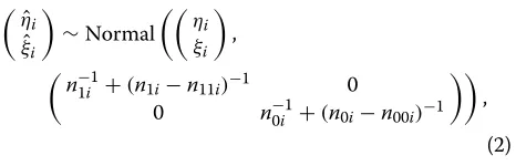
Bivariate random-effects formulation for meta-analysis Consider a meta-analysis ofndiagnostic accuracy stud-ies, each of them providing information as a two-by-two table reporting the number of true positives, true neg-atives, false positives and false negneg-atives, denoted by n11i,n00i,n10i andn01i, respectively. Let n1i be the num-ber of total positives andn0ithe number of total negatives. Consider the sensitivity (SEi) and the specificity (SPi) as diagnostic accuracy measures of study i,i = 1,. . .,n. Keeping with much of the literature, the accuracy can be expressed using the logit transformation,ηi = logit(SEi) andξi=logit(1−SPi). Given the two-by-two table infor-mation, the estimates ofSEiandSPiin studyiaren11i/n1i and n00i/n0i, respectively. Hereafter, the estimates of ηi andξiwill be denoted byηˆiandξˆi, respectively.
Models
In this paper, we will focus on the bivariate random-effects model for meta-analysis of diagnostic accuracy studies, following Reitsma et al. [7] and Arends et al. [8], among others. The model has a hierarchical structure, including a within-study level and a between-study level account-ing for the correlation between sensitivity and specificity [2–4]. Thebetween-study modelconsiders the joint distri-bution of the random effectsηiandξi,
ηi
ξi
∼Normal
η ξ
,
σ2
η ρσησξ
ρσησξ σξ2
, (1)
where η and ξ are the means over the studies, ση2 and
σ2
ξ denote the between-study variances andρis the cor-relation coefficient. As sensitivity SEi and specificitySPi tend to be negatively correlated, thenηiandξitend to be positively correlated, so thatρ >0.
Thewithin-study variabilityis accounted for at the
sec-ond stage to describe the relationship between (ηˆi,ξˆi) and (ηi,ξi). The literature distinguishes between the approximate and the exact within-study model specifica-tion. The approximate model considers(ηˆi,ξˆi)following a bivariate normal specification,
ˆ
ηi ˆ
ξi
∼Normal
ηi
ξi
,
n−1i1+(n1i−n11i)−1 0
0 n−0i1+(n0i−n00i)−1
,
(2)
ˆ
ηi ˆ
ξi
∼Normal
η ξ
,
σ2
η+n−1i1+(n1i−n11i)−1 ρσησξ
ρσησξ σξ2+n0−i1+(n0i−n00i)−1
,
the likelihood function for θ = (η,ξ,σ2
η,σξ2,ρ) has a closed-form expression and a straightforward imple-mentation using standard softwares. The model has an interesting interpretation in terms of the model suggested by Rutter and Gatsonis [22] within a Bayesian framework, with a different parameterization [23]. From a practi-cal point of view, the implementation of the bivariate Normal-Normal model is, however, more convenient [8].
The exact within-study model specification considers the observed true positives and false positives as realisa-tions of binomial variables,
n11i∼Binomial
n1i,(1+e−ηi)−1
and
n10i∼Binomial
n0i,(1+e−ξi)−1
. (3)
We refer to (1) and (3) as the Binomial-Normal
approach [16]. The resulting model is a generalised
lin-ear model, with no closed-form expression for the asso-ciated likelihood function. More computational effort is required with respect to the approximate model, as numerical integration is needed. Convergence problems represent a further drawback of the approach, with the risk of non-positive definite variance/covariance matrix and unreliable estimates of the parameters of the vari-ance/covariance matrix truncated on the boundary of the parameter space [9, 16, 19]. Both the practical issues are more severe as the number of studies decreases. The Normal-Normal approach is prone to some criticism as well, despite its feasible application. Inferential conclu-sions can be biased as a consequence of small sample size or values of sensitivity and specificity close to 1 [4, 24]. When the sample size is large, instead, there are no substantial differences between the two approaches.
Parameter estimation is typically performed via max-imum likelihood or restricted maxmax-imum likelihood [8]. The estimates of sensitivity and specificity are obtained by back-transforming the estimates ofηandξ, with stan-dard errors derived using the delta method. Alternative measures of test accuracy are the positive likelihood ratio LR+ =SE/(1−SP), the negative likelihood ratioLR− =
(1−SE)/SPand the diagnostic odds ratiodOR= {SE/(1− SE)} × {SP/(1 − SP)}. A description of the diagnostic test can be also provided by the SROC curve, through i) the characterisation of the bivariate normal model via an appropriate line and ii) the transformation of the line to the SROC space. See Arends et al. [8] for alternative specifications for the SROC curves. Discussion about the interpretation of the resulting SROC curve can be found in Hamza et al. [4] and references therein.
The measurement error problem
The hierarchical model defined for meta-analysis of diag-nostic accuracy studies is an instance of the more general bivariate meta-analysis investigated by van Houwelingen et al. [25], among others. Control rate regression [26, 27], defined as the relationship between the treatment effect and the baseline risk in meta-analysis of clinical trials, per-fectly fits the scenario we focus on in this paper. In control rate regression, attention is paid to the risk of inaccurate inferential conclusions due to the presence of measure-ment error [28, 29] affecting the treatmeasure-ment effect and the baseline risk measures. Different proposals have been sug-gested to face the measurement error problem [30–32]. Similarly, in meta-analysis of diagnostic accuracy studies the observedηˆiandξˆiare estimates of the true unknown
ηiandξiand thus they are prone to some kind of mismea-sure. Not accounting for measurement error can result in misleading inference, the most frequent being a biased estimate of the slope of the regression line used to define the SROC curve, an effect known asattenuation. See, for example, the discussion in Arends et al. [8]. The likelihood approach based of the hierarchical model given by (1)– (2) or (1)–(3) properly accounts for measurement errors [8, 26]. The within-study model (2) or (3), in fact, defines a relationship between the observed error-proneηˆi and ˆ
ξi and the unobserved corresponding ηi and ξi, in this way including the uncertainty related to the measurement process.
Despite the above mentioned analogies, control rate regression and diagnostic accuracy studies differ with respect to the role played by the variables in the regression model. In control rate regression, the baseline risk infor-mation is the covariate for the regression model using the treatment effect as response variable. In diagnostic accu-racy studies, the roles ofηi andξi in terms of response variable and covariate are not undoubtedly defined, as specificity and sensitivity can act as response or covariate according to the regression model chosen to define a par-ticular SROC curve. Only when a specific regression line used for drawing the SROC curve is defined [8], then the role of response or covariate is clearly stated.
Double SIMEX approach
In the second step, the relationship between the estimates and the amount of the added measurement error is deter-mined and used to extrapolate the corrected estimate back to the no measurement error case. The simulation step typically requires the generation of independent random variables, while the estimation can be carried out using standard simple procedures, as the least squares estima-tion or the method of moments. The extrapolaestima-tion step is a straightforward procedure. The feasibility of SIMEX application with standard software is the most attrac-tive feature explaining its wide diffusion in many areas of research. Although the approach typically considers one or more mismeasured covariates, SIMEX can easily handle situations with measurement errors on both the response and covariates, see Holcomb [34], who termed the resulting methoddouble SIMEX. This case perfectly fits the bivariate meta-analysis problem we focus on in this paper, asηˆiandξˆiare both affected by measurement error. In this way, SIMEX for diagnostic test accuracy can be thought of as an extension of Guolo [32], who investigated the methodology in control rate regression.
Let Wi = (ηˆi,ξˆi) denote the vector of the mismea-sured quantities in studyiand letXi=(ηi,ξi)denote the corresponding error-free vector. In the rest of the paper, we will focus on the approximate within-study model (2) to relate Wi and Xi. The implications of using the exact model (3) in SIMEX are illustrated in the Discussion section. The simulation step generates B datasets with additional errors starting fromWi,
Wb,i(λ)=Wi+
√
λ−1/2
i Ub,i, b=1,. . .,B,
for fixedλ ≥ 0 andi denoting the variance/covariance matrix ofWi. The additional pseudo-errorsUb,iare mutu-ally independent and normmutu-ally distributed, with zero mean and identity variance/covariance matrix. These properties are not guaranteed in finite sample as the val-ues are computer generated. A possible solution is to simulate the errors from the Gram-Schmid process [34]: the resulting pseudo-errors have the required indepen-dence properties and they are normalized to guarantee zero mean and unit variance. Moreover, their use reduces the Monte Carlo variance of the SIMEX estimates, see Section 5.3.4.1 in Carroll et al. [28]. Vector Wb,i(λ) is
aremeasurement of Wi with increasing error, such that
Wb,i(λ)=Wiforλ=0. The remeasurement is such that E(Wb,i) = Xi andVar(Wb,i) = (1+λ)iand the mean squared errorE[{Wb,i(λ)−Xi}2|Xi] equals zero forλ = −1, the key property of the simulated data. For each simu-latedb-th data set, letθˆb(λ)be the estimate ofθobtained using a standard approach, as if the measurement error was absent. The simulation step concludes with the aver-age of theBestimates for fixedλ,θ(λ)ˆ =B−1B
b=1θˆb(λ). Usuallyλassumes values on a grid , for example = {0.0, 0.5, 1.0, 1.5, 2.0}. The value of B is commonly fixed
up to 100 [20, 33]. In the extrapolation step, a relation-ship betweenθ(λ)ˆ andλis established and extrapolated back to the case of no measurement error corresponding to λ = −1. The resulting estimate is the SIMEX esti-mate θˆSIMEX. The most diffuse extrapolation function is the quadratic function, given its numerical stability, see Section 5.3.2 in Carroll et al. [28].
Lets2b(λ)be the estimated variance/covariance matrix of θ(λ)ˆ and let s2(λ) = B−1Bb=1s2b(λ). Given the sample variance/covariance matrix s2(λ) of θˆb(λ), the variance/covariance matrix of the SIMEX estimator is obtained by extrapolating back the relationship between s2(λ)−s2(λ)andλto the caseλ= −1, see Stefanski and Cook [21] and Appendix B.4 in Carroll et al. [28].
Simulation studies
Several simulation studies have been conducted to inves-tigate the performance of SIMEX and compare it to the Normal-Normal and the Binomial-Normal likelihood approaches. Data simulation follows a two-stage proce-dure. In the first stage, values forηi andξi are generated according relationship (1) or substituting the normal dis-tribution with a tdistribution with four degrees of free-dom, e.g. [9], or a skew-normal [35] distribution. In the last two cases, the robustness of the results is investigated with respect to departures from the common normality assumption for the random effects, which may some-times not be appropriate [9]. The chosen skew-normal distribution is such that the mean and the variance cor-respond to those for the normal case, but the skewness parameter for(ηi,ξi)is increased from(0, 0)(the nor-mal case) to(−1.0, 0.5) and to(−2, 2). In the second stage, the set-up is inspired by the studies in Hamza et al. [16] and Diaz [18]. The within-study numbers of true positives and false positives are simulated using rela-tionship (3). The numbers of diseased subjects n1i and nondiseased subjects n0i are generated from a uniform variable on [40, 200]. The number of studies n varies in {10; 25} in order to evaluate the methods in case of small to moderate sample sizes. Scenarios with decreas-ing accuracy are considered, namely, high accuracy
(η,ξ) = (2.94,−2.20), medium accuracy (η,ξ) =
(1.39,−1.50)and low accuracy(η,ξ)=(0.62,−0.85). Accordingly, (SEi,SPi) = (0.95, 0.90),(SEi,SPi) =
(0.80, 0.82)and(SEi,SPi)=(0.65, 0.70),i=1,. . .,n. Increasing correlation between ηi and ξi is considered,
ρ ∈ {0.2; 0.6; 0.8}. Between-study variances σ2
η and σξ2 are fixed equal to 1.2 and 0.5, respectively. One thousand datasets are generated for each combination of sample size, correlation and values of(η,ξ).
model is carried out using the restricted maximum likelihood, while inference in the Binomial-Normal model uses the maximum likelihood estimation. Likelihood maximisation, based on the Nelder and Mead algo-rithm [36], employs the method of moments estimates as starting values. SIMEX considers B = 100 remea-sured data generated using the Gram-Schmid process,
λ assuming values in = {0.0, 0.5, 1.0, 1.5, 2.0} and the quadratic extrapolation function. Parameter estima-tion within the simulaestima-tion step is based on model (2). All the methods are implemented in theRprogramming language [37].
Methods are compared with respect to bias and esti-mate of standard error of the estimators of the parameters
η,ξ,σ2
η,σξ2,ρand in terms of the 95% confidence interval for the estimators of the measures of diagnostic accuracy given by the diagnostic odds ratiodOR, the positive like-lihood ratioLR+and the negative likelihood ratio LR−. The performance of the methods in terms of convergence problems is investigated as well. Successful convergence is intended as meeting the criterion convergence (e.g., dif-ference between current and updated estimates less than 0.0001) and positive definite variance/covariance matrix. The results under non-convergence are excluded when summarising the simulation results.
Results
Simulation results
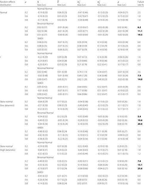
Tables 1 and 2 report the simulation results forn = 10 under the normal, thetand the skew-normal specification for(ηi,ξi), by distinguishing the high accuracy scenario and the low accuracy scenario. Results forn = 25 and results for the medium accuracy scenario are included in the Additional file 1. In all the tables, the non-convergence rate is reported in bold when larger than 5%.
Results for the high accuracy scenario (Table 1) show that, for meta-analysis with small sample size and under the random-effects normal specification, the Binomial-Normal approach appears to be preferable in terms of bias of the estimators with respect to alternative solu-tions, although at the price of a sligthly larger stan-dard error. Such a behaviour, however, deteriorates when moving to t and skewed distributions, with the bias tending to increase as the value of the correlation ρ becomes smaller. Under atrandom-effects distribution, the Binomial-Normal approach and SIMEX show an increased bias of the estimators of the variance compo-nents σ2
η and σξ2, together with an increased standard error. The effects for the Normal-Normal approach are less marked. When considering a skew-normal distribu-tion for(ηi,ξi) with a high value of skewness, SIMEX appears to be the preferable solution in terms of bias, in particular when referring to the estimates of the variance components.
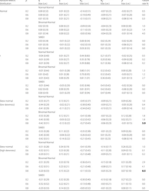
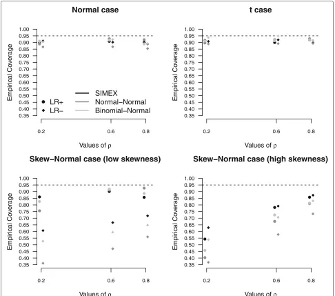
The impact of misspecification of the random-effects distribution on inferential conclusions becomes more evi-dent when computing the empirical coverage of confi-dence intervals at 95% nominal level fordOR(Fig. 1) and LR+ and LR− (Fig. 2). For dOR (Fig. 1), the Normal-Normal approach and the Binomial-Normal-Normal approach provide the less satisfactory results, with empirical cover-age probabilities far from the target 95% level, in particular when ρ is small and under a skew-normal specification for the random-effects distribution. See, for example, the extreme case ρ = 0.2 for the high-skewness scenario, with a coverage equal to 10% only for the Normal-Normal approach. Under the normal andtscenarios, the perfor-mance of the methods is comparable to that of SIMEX, with a slight underestimation of the coverage level for the Normal-Normal method. For skewed scenarios, the advantages of SIMEX over both the likelihood-based solu-tions are more marked. The empirical coverages of the confidence intervals are substantially closer to the nom-inal level, especially for large ρ. Figure 2 substantiates the results for LR+ and LR−. Under a normal or t specification for (ηi,ξi), methods are still comparable, although using the Normal-Normal likelihood method produces coverages forLR−lower than alternatives. For skewed distributions, SIMEX exhibits a more satisfactory behaviour than likelihood solutions in most of the cases when consideringLR+: for high values of ρ and a low skewness, the behaviour is comparable to the other meth-ods. ForLR−, instead, SIMEX outperforms alternatives, with empirical coverages of confidence intervals closer to the target level asρincreases.
Substantial differences between the competing methods occur in terms of failure rate of the estimation process, see the last column of Table 1. Convergence problems affect the likelihood approach, under the Binomial-Normal for-mulation in particular, in this way confirming previous findings in the literature [9, 16, 19]. The failure rate is notable whenn = 10, increases withρ and deteriorates under a skew-normal random-effects specification with high values of skewness, thus making the use of the like-lihood solution questionable. For the high skewness case andρ=0.8, for example, the Binomial-Normal approach reaches 25.6% of failures. More extreme experiments with
ρ=0.9, not reported here, substantiate the results, with a further growth of non-convergence rate higher than 31%. Conversely from the likelihood approach, the application of SIMEX does not fail in any of the examined situations, irrespectively of the sample sizen, the correlationρ and the random-effects distribution, with a non-convergence rate constantly equal to zero.
Table 1Simulation results for the high accuracy scenario
Random-effects ρ η ξ σ2
η σξ2 ρ Failure
distribution bias (s.e.) bias (s.e.) bias (s.e.) bias (s.e.) bias (s.e.) rate %
Normal-Normal
Normal 0.2 -0.19 (0.33) 0.06 (0.23) -0.47 (0.46) -0.13 (0.23) -0.04 (0.27) 2.5 0.6 -0.16 (0.33) 0.03 (0.23) -0.42 (0.47) -0.12 (0.23) -0.15 (0.22) 1.8 0.8 -0.17 (0.34) 0.02 (0.23) -0.38 (0.48) -0.10 (0.24) -0.19 (0.18) 1.8
Binomial-Normal
0.2 0.02 (0.37) -0.01 (0.24) -0.10 (0.67) -0.03 (0.28) 0.02 (0.36) 6.2 0.6 0.02 (0.38) -0.01 (0.24) -0.03 (0.71) -0.02 (0.28) -0.01 (0.28) 11.1 0.8 0.01 (0.37) -0.00 (0.24) -0.03 (0.69) -0.01 (0.29) -0.02 (0.20) 19.5
SIMEX
0.2 0.08 (0.35) -0.07 (0.25) 0.05 (0.59) 0.14 (0.30) -0.03 (0.28) 0.0 0.6 0.08 (0.35) -0.07 (0.25) 0.08 (0.59) 0.13 (0.29) -0.13 (0.23) 0.0 0.8 0.05 (0.35) -0.06 (0.25) 0.07 (0.59) 0.14 (0.30) -0.18 (0.19) 0.0
Normal-Normal
t 0.2 -0.22 (0.39) 0.09 (0.28) 0.07 (0.72) 0.16 (0.38) -0.06 (0.26) 1.6 0.6 -0.23 (0.41) 0.04 (0.28) 0.23 (0.80) 0.18 (0.38) -0.13 (0.22) 0.7 0.8 -0.20 (0.41) 0.03 (0.29) 0.21 (0.78) 0.22 (0.41) -0.17 (0.17) 0.8
Binomial-Normal
0.2 0.02 (0.46) 0.01 (0.30) 0.74 (1.13) 0.34 (0.47) -0.01 (0.33) 3.6 0.6 -0.02 (0.48) -0.01 (0.30) 0.89 (1.20) 0.36 (0.48) -0.01 (0.24) 7.9 0.8 0.00 (0.47) 0.00 (0.31) 0.82 (1.20) 0.40 (0.53) -0.03 (0.18) 14.0
SIMEX
0.2 0.05 (0.42) -0.05 (0.31) 0.64 (0.85) 0.52 (0.47) -0.05 (0.28) 0.0 0.6 -0.01 (0.43) -0.07 (0.31) 0.77 (0.90) 0.51 (0.47) -0.10 (0.22) 0.0 0.8 0.00 (0.42) -0.05 (0.31) 0.66 (0.86) 0.52 (0.47) -0.15 (0.17) 0.0
Normal-Normal
Skew-normal 0.2 -0.64 (0.29) 0.17 (0.22) -0.54 (0.38) -0.13 (0.22) 0.03 (0.26) 1.4 (low skewness) 0.6 -0.57 (0.30) 0.00 (0.23) -0.49 (0.40) -0.13 (0.23) -0.11 (0.21) 1.8 0.8 -0.52 (0.31) -0.10 (0.23) -0.44 (0.43) -0.13 (0.22) -0.17 (0.17) 2.1
Binomial-Normal
0.2 -0.54 (0.32) 0.12 (0.23) -0.35 (0.48) -0.05 (0.26) 0.10 (0.33) 5.4 0.6 -0.49 (0.32) -0.05 (0.24) -0.28 (0.53) -0.03 (0.28) 0.03 (0.26) 10.6 0.8 -0.44 (0.34) -0.16 (0.24) -0.18 (0.59) -0.02 (0.29) 0.00 (0.19) 20.0
SIMEX
0.2 -0.48 (0.32) 0.06 (0.24) -0.16 (0.48) 0.11 (0.28) 0.05 (0.27) 0.0 0.6 -0.42 (0.33) -0.11 (0.25) -0.10 (0.51) 0.13 (0.29) -0.09 (0.22) 0.0 0.8 -0.38 (0.33) -0.22 (0.25) -0.04 (0.54) 0.13 (0.30) -0.16 (0.18) 0.0
Normal-Normal
Skew-normal 0.2 -0.59 (0.30) 0.37 (0.20) -0.52 (0.40) -0.19 (0.18) 0.20 (0.23) 1.2 (high skewness) 0.6 -0.44 (0.31) 0.24 (0.22) -0.44 (0.43) -0.15 (0.21) 0.01 (0.18) 1.8 0.8 -0.32 (0.32) 0.15 (0.22) -0.43 (0.44) -0.13 (0.21) -0.11 (0.15) 1.2
Binomial-Normal
0.2 -0.49 (0.32) 0.35 (0.21) -0.30 (0.51) -0.13 (0.21) 0.30 (0.29) 7.6 0.6 -0.33 (0.35) 0.22 (0.23) -0.14 (0.62) -0.06 (0.26) 0.16 (0.20) 15.1 0.8 -0.19 (0.37) 0.13 (0.24) -0.08 (0.66) -0.04 (0.27) 0.05 (0.16) 25.6
SIMEX
0.2 -0.43 (0.32) 0.31 (0.21) -0.13 (0.50) -0.02 (0.22) 0.22 (0.24) 0.0 0.6 -0.26 (0.34) 0.17 (0.23) 0.00 (0.55) 0.06 (0.26) 0.03 (0.19) 0.0 0.8 -0.14 (0.35) 0.08 (0.24) 0.02 (0.57) 0.09 (0.27) -0.10 (0.16) 0.0
Bias and average of the estimated standard errors (s.e.) for the estimators ofη,ξ,σ2
Table 2Simulation results for the low accuracy scenario
Random-effects ρ η ξ σ2
η σξ2 ρ Failure
distribution bias (s.e.) bias (s.e.) bias (s.e.) bias (s.e.) bias (s.e.) rate % Normal-Normal
Normal 0.2 0.00 (0.32) 0.01 (0.22) -0.16 (0.51) -0.07 (0.22) -0.02 (0.27) 0.5 0.6 0.00 (0.32) 0.01 (0.21) -0.19 (0.49) -0.09 (0.21) -0.07 (0.20) 0.0 0.8 0.01 (0.33) 0.01 (0.21) -0.15 (0.51) -0.08 (0.21) -0.08 (0.14) 0.3
Binomial-Normal
0.2 0.02 (0.33) 0.00 (0.22) -0.09 (0.54) -0.04 (0.23) 0.00 (0.30) 1.0 0.6 0.00 (0.33) 0.00 (0.22) -0.11 (0.53) -0.05 (0.23) -0.01 (0.22) 1.4 0.8 0.01 (0.34) 0.00 (0.22) -0.05 (0.56) -0.04 (0.23) -0.01 (0.14) 4.0
SIMEX
0.2 0.03 (0.34) -0.01 (0.22) 0.00 (0.54) 0.02 (0.24) -0.02 (0.28) 0.0 0.6 0.01 (0.33) -0.01 (0.22) -0.02 (0.53) 0.01 (0.23) -0.06 (0.21) 0.0 0.8 0.02 (0.34) -0.01 (0.22) 0.03 (0.55) 0.01 (0.23) -0.07 (0.14) 0.0
Normal-Normal
t 0.2 -0.04 (0.40) 0.01 (0.27) 0.44 (0.83) 0.21 (0.37) -0.02 (0.25) 0.5 0.6 -0.01 (0.39) 0.03 (0.27) 0.35 (0.78) 0.20 (0.36) -0.09 (0.20) 0.2 0.8 -0.01 (0.39) 0.02 (0.27) 0.39 (0.80) 0.21 (0.36) -0.08 (0.14) 0.2
Binomial-Normal
0.2 -0.01 (0.44) -0.01 (0.28) 0.80 (1.01) 0.32 (0.42) 0.00 (0.28) 1.3 0.6 0.01 (0.42) 0.01 (0.28) 0.70 (0.95) 0.32 (0.42) -0.03 (0.21) 1.2 0.8 -0.01 (0.43) 0.00 (0.29) 0.81 (1.01) 0.36 (0.43) -0.01 (0.13) 2.7
SIMEX
0.2 -0.01 (0.44) -0.03 (0.29) 0.92 (0.96) 0.43 (0.42) -0.02 (0.26) 0.0 0.6 0.02 (0.43) 0.00 (0.29) 0.81 (0.91) 0.42 (0.42) -0.08 (0.20) 0.0 0.8 0.00 (0.43) -0.01 (0.29) 0.87 (0.94) 0.47 (0.44) -0.07 (0.13) 0.0
Normal-Normal
Skew-normal 0.2 -0.55 (0.27) 0.13 (0.21) -0.45 (0.37) -0.09 (0.21) 0.09 (0.26) 1.0 (low skewness) 0.6 -0.44 (0.29) -0.02 (0.21) -0.38 (0.40) -0.09 (0.21) -0.05 (0.20) 0.4 0.8 -0.41 (0.29) -0.11 (0.21) -0.34 (0.42) -0.10 (0.21) -0.09 (0.14) 0.2
Binomial-Normal
0.2 -0.55 (0.28) 0.12 (0.21) -0.41 (0.38) -0.07 (0.22) 0.12 (0.28) 1.8 0.6 -0.45 (0.30) -0.03 (0.22) -0.32 (0.42) -0.06 (0.23) 0.02 (0.21) 1.8 0.8 -0.42 (0.31) -0.12 (0.22) -0.27 (0.45) -0.06 (0.23) -0.01 (0.15) 5.9
SIMEX
0.2 -0.55 (0.28) 0.11 (0.22) -0.35 (0.38) -0.01 (0.22) 0.09 (0.26) 0.0 0.6 -0.45 (0.30) -0.04 (0.22) -0.26 (0.42) 0.01 (0.23) -0.04 (0.20) 0.0 0.8 -0.42 (0.31) -0.14 (0.22) -0.21 (0.45) 0.01 (0.23) -0.08 (0.14) 0.0
Normal-Normal
Skew-normal 0.2 -0.51 (0.28) 0.34 (0.19) -0.41 (0.39) -0.16 (0.17) 0.26 (0.22) 1.0 (high skewness) 0.6 -0.32 (0.31) 0.23 (0.20) -0.27 (0.45) -0.11 (0.20) 0.09 (0.15) 0.1 0.8 -0.20 (0.31) 0.15 (0.21) -0.21 (0.48) -0.09 (0.21) -0.01 (0.11) 0.2
Binomial-Normal
0.2 -0.51 (0.29) 0.33 (0.19) -0.36 (0.41) -0.15 (0.18) 0.31 (0.20) 2.9
0.6 -0.32 (0.31) 0.23 (0.21) -0.21 (0.48) -0.08 (0.21) 0.17 (0.16) 4.1
0.8 -0.20 (0.33) 0.15 (0.22) -0.11 (0.53) -0.05 (0.23) 0.07 (0.10) 8.5
SIMEX
0.2 -0.51 (0.29) 0.32 (0.20) -0.30 (0.40) -0.10 (0.18) 0.27 (0.22) 0.0
0.6 -0.32 (0.32) 0.22 (0.21) -0.13 (0.48) -0.03 (0.21) 0.11 (0.15) 0.0
0.8 -0.20 (0.33) 0.14 (0.22) -0.05 (0.52) -0.01 (0.22) 0.00 (0.11) 0.0
Bias and average of the estimated standard errors (s.e.) for the estimators ofη,ξ,σ2
Normal case
Values of ρ
Empir
ical Co
v
e
rage
0.2 0.6 0.8
0.10 0.15 0.20 0.25 0.30 0.35 0.40 0.45 0.50 0.55 0.60 0.65 0.70 0.75 0.80 0.85 0.90 0.95 1.00
SIMEX
Normal−Normal
Binomial−Normal
t case
Values of ρ
Empir
ical Co
v
e
rage
0.2 0.6 0.8
0.10 0.15 0.20 0.25 0.30 0.35 0.40 0.45 0.50 0.55 0.60 0.65 0.70 0.75 0.80 0.85 0.90 0.95 1.00
Skew−Normal case (low skewness)
Values of ρ
Empir
ical Co
v
e
rage
0.2 0.6 0.8
0.10 0.15 0.20 0.25 0.30 0.35 0.40 0.45 0.50 0.55 0.60 0.65 0.70 0.75 0.80 0.85 0.90 0.95 1.00
Skew−Normal case (high skewness)
Values of ρ
Empir
ical Co
v
e
rage
0.2 0.6 0.8
0.10 0.15 0.20 0.25 0.30 0.35 0.40 0.45 0.50 0.55 0.60 0.65 0.70 0.75 0.80 0.85 0.90 0.95 1.00
Fig. 1Diagnostic odds ratio results. Empirical coverages of confidence intervals for diagnostic odds ratio under increasing values ofρ, on the basis of 1, 000 replicates for the high accuracy scenario, withn=10
only slightly reduced with respect to Table 1. The most interesting result is the reduction of the failure rate with respect to the high accuracy scenario. With regards to the likelihood analysis, the most substantial reduction of non-convergences is observed for the Binomial-Normal formulation, whose failure rate does not exceed the 5% level under the normal or trandom-effects formulation and reaches 8.5% under the skew-normal distribution. Similarly to the high accuracy context, the failure rate tends to increase withρ. SIMEX maintains a failure rate equal to zero.
Results for the medium accuracy scenario are reported in Additional file 1. Conclusions are coherent wth those
from the low and high accuracy scenario. From a compu-tational point of view, non-convergence problems mainly affect the Binomial-Normal approach, with failure rates reaching 22.3% under the skew-normal specification when the sample size is small.
Normal case
Values of ρ
Empir
ical Co
v
e
rage
0.2 0.6 0.8
0.35 0.40 0.45 0.50 0.55 0.60 0.65 0.70 0.75 0.80 0.85 0.90 0.95 1.00
LR+ LR−
SIMEX
Normal−Normal Binomial−Normal
t case
Values of ρ
Empir
ical Co
v
e
rage
0.2 0.6 0.8
0.35 0.40 0.45 0.50 0.55 0.60 0.65 0.70 0.75 0.80 0.85 0.90 0.95 1.00
Skew−Normal case (low skewness)
Values of ρ
Empir
ical Co
v
e
rage
0.2 0.6 0.8
0.35 0.40 0.45 0.50 0.55 0.60 0.65 0.70 0.75 0.80 0.85 0.90 0.95 1.00
Skew−Normal case (high skewness)
Values of ρ
Empir
ical Co
v
e
rage
0.2 0.6 0.8
0.35 0.40 0.45 0.50 0.55 0.60 0.65 0.70 0.75 0.80 0.85 0.90 0.95 1.00
Fig. 2Positiveandnegativelikelihood ratio results. Empirical coverages of confidence intervals forpositiveandnegativelikelihood ratio under increasing values ofρ, on the basis of 1, 000 replicates for the high accuracy scenario, withn=10
the simulation settings. The Binomial-Normal approach substantially reduces the number of failures, with just two cases exceeding the 5% threshold, corresponding to the skew-normal case with high skewness andρ =0.8 in the high accuracy and medium accuracy scenarios. SIMEX maintains a failure rate equal to zero.
Data example
Van Zaane et al. [38] perform a meta-analysis of six diag-nostic accuracy studies for the assessment of atheroscle-rosis in the ascending aorta in patients undergoing cardiac surgery through transesophageal echocardiogra-phy in place of the reference-standard method given by
epiaortic ultrasound scanning. The available information is reported in Table 3. Data have been recently re-analysed in Zapf et al. [15] through a nonparametric approach.
Table 3Transesophageal echocardiography data [38]
Study TP FP TN FN
1 3 0 72 25
2 3 0 66 19
3 4 0 56 10
4 0 0 8 6
5 4 1 66 10
6 5 1 49 11
Data includes true positives (TP), false positives (FP), true negatives (TN), false negatives (FN)
Zapf et al. [15], the likelihood analysis using the Binomial-Normal specification does not converge and the likelihood estimation of the correlationρis on the boundary of the parameter space, equal to 1. These results coincide with those available from our implementation of the likelihood approach. Changing the optimization algorithm and the starting values does not solve the non-convergence prob-lem. The application of SIMEX, conversely, does not pose any convergence issue. The estimates of ηandξ result-ing in−1.525 (standard error 0.292) and−4.266 (standard error 0.325), respectively, give rise to the estimates of sensitivity and specificity as reported in Table 4. SIMEX-based confidence intervals for sensitivity and specificity are narrower than those available from the Normal-Normal approach. The results from the nonparametric approach of Zapf et al. [15], close to those from SIMEX, are reported for completeness.
Discussion
Results from the simulation studies indicate that SIMEX leads to satisfactory inferential results in a wide range of scenarios. When the normality assumption for the random-effects distribution holds, the method is compa-rable to the likelihood solutions in terms of bias and esti-mated standard error of the estimators of the parameters of interest and slightly superior to the Binomial-Normal formulation in terms of empirical coverages of confi-dence intervals for different diagnostic accuracy mea-sures. When departures from the normality assumptions hold in terms of low or high skewness, then advantages
Table 4Data analysis
Method Sensitivity Specificity
Normal-Normal model 21 (13, 32) 99 (96, 99)
Binomial-Normal model – –
SIMEX approach 17.9 (10.9, 27.8) 98.6 (97.4, 99.3)
Nonparametric model (Zapf et al. [15]) 19.0 (11.9, 28.9) 99.4 (97.9, 99.8)
Estimates and 95% confidence intervals (in parentheses) for sensitivity and specificity obtained from different methods for the analysis of transesophageal echocardiography data [38]. Results are multiplied by 100
of using SIMEX are much more evident. In particular, empirical coverages of confidence intervals for the diag-nostic accuracy measures are closer to the 95% target level than alternatives. The likelihood approach under the Binomial-Normal formulation shows a less satisfactory performance.
A substantial difference between SIMEX and the like-lihood approach is in terms of failure rate of conver-gence. SIMEX has not convergence problems whichever the examined scenario. Conversely, likelihood solutions suffer for convergence difficulties, especially in case of skewed random-effects distribution. The highest levels of failure rate are reached using the Binomial-Normal formulation and they are much more frequent as the sample size is small and the value of the correlation ρ increases. Simulation results are in accordance with pre-vious findings in the literature about convergence issues and numerical instabilities of the likelihood approach. Possible solutions evaluated in the simulation studies, including the change of the optimisation algorithm and the change of the starting values [16, 19], only slightly reduce the number of failures. When adopting the SIMEX strategy, several solutions are available in case of con-vergence failure, although we did not experience such a problem in our study. Possible solutions include the choice of a different estimation method within eachb-th replication of the simulation step or varying the number of simulated datasets B. An additional practical strat-egy is the visual inspection of the SIMEX components and the direct extrapolation of the points of interest. This strategy is suggested in Section B.4.1 of Carroll et al. [28] when the SIMEX estimated variance/covariance matrix is non-positive definite. Although possible, this is an infrequent case and we did not encounter it in our simulations.
From a strictly practical point of view, the implementa-tion of SIMEX, despite its simulaimplementa-tion-based nature, is not involved neither time-consuming and can proceed by tak-ing advantage of simple estimation methods, such as the method of moments. TheR[37] code for SIMEX imple-mentation is made available in the Additional file 2 and illustrated in the Additional file 3.
Although the scenarios investigated in the paper do not consider the presence of additional level covariates in model (1), SIMEX can be extended to account for them. In this case, the number of remeasured datasetsBis recom-mended to be increased in order to guarantee the results having an acceptable precision, see Section 5.3 in Carroll et al. [28].
empirical investigations with different correction values show that the 0.5 correction does not impact the results. Such a behaviour is related to the SIMEX procedure, as the correction can affect only the original data, while the remeasured data of the simulation step are not influenced. Simulating the discrete components of the two-by-two table in place of their continuous logit transformations
ˆ
ηi andξˆi is theoretically possible. In this case, the mea-surement error problem affects the classification of the positive/negative results in the two-by-two table, thus being called misclassification problem, see Küchenhoff et al. [39]. However, moving from the new generated dis-crete data to the logit transformations would still be an obligatory step, as the data are necessary for inference in the main model (1). In this case, the 0.5 correction would still apply, not only on the original data but in every case the problem arises within the simulation step. How to circumvent these limitations when simulating from the exact model (3) represents a topic of future research.
Conclusions
This paper focused on bivariate random-effects models for meta-analysis of diagnostic test accuracy. Attention is paid to the presence of errors affecting the measures of diagnostic accuracy. Standard likelihood-based proce-dures are shown to be prone to several drawbacks, despite their wide diffusion. The inaccuracy of inferential conclu-sions for small sample size and in case of misspecifica-tion of the random-effects distribumisspecifica-tion is accompanied by computational issues which seriously affect the applicabil-ity of the approach. The SIMEX methodology represents an interesting and promising alternative. Reliable infer-ence properly accounting for the presinfer-ence of measure-ment errors is obtained with neither computational effort not numerical instabilities. The satisfactory performance of SIMEX illustrated through extensive simulation exper-iments is not affected by study characteristics, such as sample size or measurement error correlation. Robustness to departures from normal random-effects distributions is a substantial improvement over standard likelihood solu-tions. The availability of the R code for a user-friendly implementation of SIMEX is aimed at encouraging its use.
Additional files
Additional file 1:The file includes a portion of the simulation results comparing the performance of SIMEX and likelihood-based approaches in the medium accuracy scenario and in the low and high accuracy scenarios for sample sizen=25. (PDF 91 kb)
Additional file 2:Rcode for applying the SIMEX approach. (R 10.2 kb)
Additional file 3:The file illustrates how to apply SIMEX for data analysis using theRcode available in Additional file 2. (PDF 64.4 kb)
Abbreviations
dOR: Diagnostic odds ratio; FN: False negatives; FP: False positives; LR-: Negative likelihood ratio; LR+: Positive likelihood ratio; s.e.: Standard error; SE: Sensitivity; SIMEX: Simulation extrapolation; SP: Specificity; SROC: Summary operating receiver characteristic; TN: True negatives; TP: True positives
Acknowledgments
Not applicable.
Funding
This work was supported by a grant from the University of Padova (Progetti di Ricerca di Ateneo 2015, CPDA153257).
Availability of data and materials
The real data used for the illustration of SIMEX and likelihood procedures are reported in Table 3. TheRcode to implement SIMEX is available in the Additional file 2 and the commands needed to apply the software for data analysis are illustrated in the Additional file 3.
Competing interests
The author declares that she has no competing interests.
Consent for publication
Not applicable.
Ethics approval and consent to participate
Not applicable.
Received: 18 August 2016 Accepted: 22 December 2016
References
1. Honest H, Khan K. Reporting of measures of accuracy in systematic reviews of diagnostic literature. BMC Health Serv Res. 2002;2:4:266–7. 2. Riley RD, Abrams KR, Sutton AJ, Lambert PC, Thompson JR. Bivariate
random-effects meta-analysis and the estimation of between-study correlation. BMC Med Res Methodol. 2007;7:3:266–7.
3. Riley RD, Thompson JR, Abrams KR. An alternative model for bivariate random-effects meta-analysis when the within-study correlations are unknown. Biostatistics. 2008;9:172–86.
4. Hamza TH, van Houwelingen HC, Stijnen T. The binomial distribution of meta-analysis was preferred to model within-study variability. J Clin Epidemiol. 2008;61:41–51.
5. Littenberg B, Moses LE. Estimating diagnostic-accuracy from multiple conflicting reports: a new meta-analytic method. Med Dec Making. 1993;13:313–21.
6. Moses LE, Shapiro D, Littenberg B. Combining independent studies of a diagnostic test into a summary ROC curve: data-analytic approaches and some additional considerations. Stat Med. 1993;12:1293–316.
7. Reitsma JB, Glas AS, Rutjes AWS, Scholten RJ, Bossuyt PM, Zwinderman AH. Bivariate analysis of sensitivity and specificity produces informative summary measures in diagnostic reviews. J Clin Epidemiol. 2005;58: 982–90.
8. Arends LR, Hamza TH, van Houwelingen HC, Heijenbrok-Kal MH, Hunink MGM, Stijnen T. Bivariate random effects meta-analysis of ROC curves. Med Dec Making. 2008;28:621–38.
9. Chen Y, Liu Y, Ning J, Nie L, Zhu H, Chu H. A composite likelihood method for bivariate meta-analysis in diagnostic systematic reviews. Stat Methods Med Res. 2014. http://journals.sagepub.com/doi/full/10.1177/ 0962280214562146.
10. Chu H, Nie L, Chen Y, Huang Y, Sun W. Bivariate random effects models for meta-analysis of comparative studies with binary outcomes: methods for the absolute risk difference and relative risk. Stat Methods Med Res. 2012;21:621–33.
11. Kuss O, Hoyer A, Solms A. Meta-analysis for diagnostic accuracy studies: a new statistical model using beta-binomial distributions and bivariate copulas. Stat Med. 2014;33:17–30.
13. Eusebi P, Reitsma JB, Vermunt JK. Latent class bivariate model for the meta-analysis of diagnostic test accuracy studies. BMC Med Res Methodol. 2014;14:88:.
14. Schlattmann P, Verba M, Dewey M, Walther M. Mixture models in diagnostic meta-analyses – clustering summary receiver operating characteristic curves accounted for heterogeneity and correlation. J Clin Epidemiol. 2015;68:61–72.
15. Zapf A, Hoyer A, Kramer K, Kuss O. Nonparametric meta-analysis for diagnostic accuracy studies. Stat Med. 2015;34:3831–41.
16. Hamza TH, Reitsma JB, Stijnen T. Meta-analysis of diagnostic studies: A comparison of random intercept, normal-normal, and binomial-normal bivariate summary ROC approaches. Med Dec Making. 2008;28:639–49. 17. Paul M, Riebler A, Bachmann LM, Rue H, Held L. Bayesian bivariate
meta-analysis of diagnostic test studies using integrated nested Laplace approximations. Stat Med. 2010;29:1325–9.
18. Diaz M. Performance measures of the bivariate random effects model for meta-analyses of diagnostic accuracy. Comput Stat Data Anal. 2015;83: 82–90.
19. Takwoingi Y, Guo B, Riley RD, Deeks JJ. Performance of methods for meta-analysis of diagnostic test accuracy with few studies or sparse data. Stat Methods Med Res. 2015. http://journals.sagepub.com/doi/abs/10. 1177/0962280215592269?url_ver=Z39.88-2003&rfr_id=ori:rid:crossref. org&rfr_dat=cr_pub%3dpubmed.
20. Cook JR, Stefanski LA. Simulation extrapolation estimation in parametric measurement error models. J Am Stat Assoc. 1994;89:1314–28. 21. Stefanski LA, Cook JR. Simulation-extrapolation: the measurement error
jackknife. J Am Stat Assoc. 1995;90:1247–56.
22. Rutter CM, Gatsonis CA. A hierarchical regression approach to meta-analysis of diagnostic test accuracy evaluations. Stat Med. 2001;20: 2865–84.
23. Harbord RM, Deeks JJ, Egger M, Whiting P, Sterne JA. A unification of models for meta-analysis of diagnostic accuracy studies. Biostatistics. 2007;8:239–51.
24. Chu H, Cole SR. Bivariate meta-analysis of sensitivity and specificity with sparse data: a generalized linear mixed model approach. J Clin Epidemiol. 2006;59:1331–3.
25. Van Houwelingen HC, Arends LR, Stijnen T. Advanced methods in meta-analysis: multivariate approach and meta-regression. Stat Med. 2002;21:589–624.
26. McIntosh MW. The population risk as an explanatory variable in research synthesis of clinical trials. Stat Med. 1996;15:1713–28.
27. Schmid CH, Lau J, McIntosh MW, Cappelleri JC. An empirical study of the effect of the control rate as a predictor of treatment efficacy in
meta-analysis of clinical trials. Stat Med. 1998;17:1923–42.
28. Carroll RJ, Ruppert D, Stefanski LA, Crainiceanu C. Measurement Error in Nonlinear Models: A Modern Perspective. Boca Raton: Chapman & Hall, CRC Press; 2006.
29. Buonaccorsi JP. Measurement Error: Models, Methods and Applications. Boca Raton: Chapman & Hall, CRC Press; 2010.
30. Arends LR, Hoes AW, Lubsen J, Grobbee DE, Stijnen T. Baseline risk as predictor of treatment benefit: three clinical meta-re-analyses. Stat Med. 2000;19:3497–518.
31. Ghidey W, Stijnen T, van Houwelingen HC. Modelling the effect of baseline risk in meta-analysis: A review from the perspective of errors-in-variables regression. Stat Methods Med Res. 2013;22:307–23. 32. Guolo A. The SIMEX approach to measurement error correction in
meta-analysis with baseline risk as covariate. Stat Med. 2014;33:2062–76. 33. Carroll RJ, Küchenhoff H, Lombard F, Stefanski LA. Asymptotics for the
SIMEX estimator in nonlinear measurement error models. J Am Stat Assoc. 1996;91:242–50.
34. Holcomb J. Regression with covariates and outcome calculated from a common set of variables measured with error: Estimation using the SIMEX method. Stat Med. 1999;18:2847–62.
35. Azzalini A. A class of distributions which includes the normal ones. Scand J Stat. 1985;12:171–8.
36. Nelder JA, Mead R. A simplex algorithm for function minimization. Scand J Stat. 1965;7:308–13.
37. R Core Team: R: A language and environment for statistical computing. Vienna, Austria: R Foundation for Statistical Computing; 2015. http:// www.R-project.org/.
38. Van Zaane B, Zuithoff NPA, Reitsma JB, Bax L, Nierich AP, Moons KG. Meta-analysis of the diagnostic accuracy of transesophageal echocardiography for assessment of atherosclerosis in the ascending aorta in patients undergoing cardiac surgery. Acta Anaesthesiol Scand. 2008;52:1179–87.
39. Küchenhoff H, Mwalili SM, Lesaffre E. A general method for dealing with misclassification in regression: The misclassification SIMEX. Biometrics. 2006;62:85–96.
• We accept pre-submission inquiries
• Our selector tool helps you to find the most relevant journal
• We provide round the clock customer support
• Convenient online submission
• Thorough peer review
• Inclusion in PubMed and all major indexing services
• Maximum visibility for your research
Submit your manuscript at www.biomedcentral.com/submit
![Table 3 Transesophageal echocardiography data [38]](https://thumb-us.123doks.com/thumbv2/123dok_us/9317762.1919075/10.595.57.293.633.705/table-transesophageal-echocardiography-data.webp)
