Http://www.ijetmr.com©International Journal of Engineering Technologies and Management Research [249]
COMPRESSIVE SENSING
Abhilasha Sharma *1
*1
Assistant professor, Department of Electronics Engineering, Madhav Institute of Technology & Science Gwalior (M.P)-474005, India
Abstract:
Compressive sensing is a relatively new technique in the signal processing field which allows acquiring signals while taking few samples. It works on two principles: sparsity, which pertains to the signals of interest, and incoherence, which pertains to the sensing modality. Since, in conventional system all signals follow the Nyquist criteria, in which the sampling rate must be at least twice the maximum frequency of modulating signal. But, in this new concept we can recover the signal below the Nyquist rate. This paper presents the basic concept of compressive sensing and area of applications, where we can apply this technique.
Keywords: Compressive Sensing; Sparsity; L1-Norm.
Cite This Article: Abhilasha Sharma. (2018). “COMPRESSIVE SENSING.” International
Journal of Engineering Technologies and Management Research, 5(2:SE), 249-259. DOI:
https://doi.org/10.29121/ijetmr.v5.i2.2018.655.
1. Introduction
Compressed sensing is a signal processing technique for efficiently acquiring and reconstructing a signal, by finding solutions to underdetermine linear systems. This takes advantage of the signal's sparseness or compressibility in some domain, allowing the entire signal to be determined from relatively few measurements. In recent years, compressed sensing (CS) has attracted considerable attention in areas of applied mathematics, computer science, and electrical engineering by suggesting that it may be possible to surpass the traditional limits of sampling theory [1]. CS builds upon the fundamental fact that we can represent many signals using only a few non-zero coefficients in a suitable basis or dictionary.
Since, in conventional system all signals follow the Nyquist criteria, in which the sampling rate must be at least twice the maximum frequency of modulating signal. But, in this new concept that is developed by Emmanuel Candes, Terence Tao and David Donoho around the year 2004, we can acquire the signal below the Nyquist rate. [2]
Http://www.ijetmr.com©International Journal of Engineering Technologies and Management Research [250] A signal is said to be sparse if it contain mostly zeros, and only a few non-zero elements. If signals have non-zero elements, it is called s-sparse.
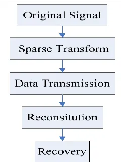
Figure 1: the framework of compressed sensing
2. Principle of Compressive Sensing
Compressed sensing (CS) has emerged as a new framework for signal acquisition and sensor design. CS enables a potentially large reduction in the sampling and computation costs for sensing signals that have a sparse or compressible representation. While the Nyquist-Shannon sampling theorem states that a certain minimum number of samples is required in order to perfectly capture an arbitrary band limited signal, when the signal is sparse in a known basis we can vastly reduce the number of measurements that need to be stored. Consequently, when sensing sparse signals we might be able to do better than suggested by classical results. This is the fundamental idea behind CS: rather than first sampling at a high rate and then compressing the sampled data, we would like to find ways to directly sense the data in a compressed form | i.e., at a lower sampling rate. To make this possible, CS relies on two principles: sparsity and incoherence [3].
2.1.Sparsity
Sparsity expresses the idea that the ―information rate‖ of a continuous time signal may be much smaller than suggested by its bandwidth, or that a discrete-time signal depends on a number of degrees of freedom which is comparably much smaller than its (finite) length. More precisely, CS exploits the fact that many natural signals are sparse or compressible in the sense that they have concise representations when expressed in the proper basis Ψ.
2.2.Incoherence
Http://www.ijetmr.com©International Journal of Engineering Technologies and Management Research [251] differently, incoherence says that unlike the signal of interest, the sampling/sensing waveforms have an extremely dense representation in Ψ.
3. Compressible Signals
An important assumption used in the context of compressive sensing (CS) is that signals exhibit a degree of structure. So far the only structure we have considered is sparsity [4], i.e., the number of non-zero values the signal has when representation in an orthonormal basis [5]. The signal is considered sparse if it has only a few nonzero values in comparison with its overall length.
Few structured signals are truly sparse; rather they are compressible. A signal is compressible if its sorted coefficient magnitudes in Ψ decay rapidly. To consider this mathematically, let x be a signal which is compressible in the basis Ψ:
x = Ψα, (1)
Where α are the coefficients of x in the basis Ψ. If x is compressible, then the magnitudes of the sorted coefficients αs observe a power law decay:
| αs |≤C1s-q , s = 1, 2,…. (2)
We define a signal as being compressible if it obeys this power law decay. The larger q is, the faster the magnitudes decay, and a signal is more compressible. Because the magnitudes of coefficients decay so rapidly, compressible signals can be represented well by K N coefficients. The best K-term approximation of a signal is the one in which the K largest coefficients are kept, with the rest being zero. The error between the true signal and its K term approximation is denoted the K-term approximation error σK (x), defined as
(3)
For compressible signals, we can establish a bound with power law decay as follows:
σK(x) C2K(1/2-s) (4)
In fact, one can show that σK(x) 2 will decay as K-r if and only if the sorted coefficients αi decay as i-r+1/2
4. Norms
Http://www.ijetmr.com©International Journal of Engineering Technologies and Management Research [252] 4.1.L0-Norm
The first norm we are going to discuss is a L0-norm. By definition, L0-norm of x is
||x||0 = 0√ (Σi xi0)
Strictly speaking, L0-norm is not actually a norm. It is a cardinality function which has its definition in the form of LPnorm, though many people call it a norm. It is a bit tricky to work with because there is a presence of zeroth-power and zeroth-root in it. Obviously any x>0 will become one, but the problems of the definition of zeroth-power and especially zeroth-root is messing things around here. So in reality, most mathematicians and engineers use this definition of L0-norm instead:
||x||0 = # (i| xi ≠ 0)
that is a total number of non-zero elements in a vector.
Because it is a number of non-zero elements, there are so many applications that use L0-norm. Lately it is even more in focus because of the rise of the Compressive Sensing scheme, which is try to find the sparsest solution of the underdetermined linear system. The sparsest solution means the solution which has fewest non-zero entries, i.e. the lowest L0-norm. This problem is usually regarding as an optimization problem of L0-norm or L0-optimisation.
4.1.1. L0-Optimisation
Many applications, including Compressive Sensing, try to minimize the L0-norm of a vector corresponding to some constraints, hence called ―L0-minimisation‖. A standard minimization problem is formulated as:
min ||x||0 subject to Ax=b
However, doing so is not an easy task. Because the lack of L0-norm’s mathematical representation, L0- minimisation is regarded by computer scientist as an NP-hard problem, simply says that it’s too complex and almost impossible to solve.
In many case, L0-minimisation problem is relaxed to be higher-order norm problem such as L1-minimisation and L2-L1-minimisation.
4.2.L1-Norm
Following the definition of norm, L1-norm of x is defined as
||x||1 = Σi |xi|
Http://www.ijetmr.com©International Journal of Engineering Technologies and Management Research [253] SAD(x1, x2) = || x1-x2||1 = Σ |x1i - x2i|
It is called Sum of Absolute Difference (SAD) among computer vision scientists.
In more general case of signal difference measurement, it may be scaled to a unit vector by:
Where n is a size of x.
Which is known as Mean-Absolute Error (MAE).
4.3.L2-Norm
The most popular of all norms is the L2-norm. It is used in almost every field of engineering and science as a whole. Following the basic definition, L2-norm is defined as
||x||2 = √ (Σ i xi2)
L2-norm is well known as a Euclidean norm, which is used as a standard quantity for measuring a vector difference. As in L1-norm, if the Euclidean norm is computed for a vector difference, it is known as a Euclidean distance:
||x1-x2||2= √ (Σi(x1i - x2i) 2)
Or in its squared form, known as a Sum of Squared Difference (SSD) among Computer Vision scientists:
It’s most well-known application in the signal processing field is the Mean-Squared Error (MSE) measurement, which is used to compute a similarity, a quality, or a correlation between two signals. MSE is
As previously discussed in L0-optimisation section, because of many issues from both a computational view and a mathematical view, many L0-optimisation problems relax themselves to become L1– and L2-optimisation instead.
4.3.1. L2-optimisation
Http://www.ijetmr.com©International Journal of Engineering Technologies and Management Research [254] min ||x||2 subject to Ax=b
Assume that the constraint matrix A has full rank; this problem is now an underdetermined system which has infinite solutions. The goal in this case is to draw out the best solution, i.e. has lowest L2-norm, from these infinitely many solutions. This could be a very tedious work if it was to be computed directly. Luckily it is a mathematical trick that can help us a lot in this work.
By using a trick of Lagrange multipliers, we can then define a Lagrangian
Where λ is the introduced Lagrange multiplier. Take derivative of this equation equal to zero to find an optimal solution and get
Plug This Solution into the Constraint To Get
And finally
By using this equation, we can now instantly compute an optimal solution of the L2-optimisation problem. This equation is well known as the Moore-Penrose Pseudoinverse and the problem itself is usually known as Least Square problem, Least Square regression, or Least Square optimisation.
However, even though the solution of Least Square method is easy to compute, it’s not necessary be the best solution. Because of the smooth nature of L2-norm itself, it is hard to find a single, best solution for the problem.
In contrary, the L1-optimisation can provide much better result than this solution.
4.3.2. L1-optimisation
As usual, the L1-minimisation problem is formulated as
Http://www.ijetmr.com©International Journal of Engineering Technologies and Management Research [255] Because the nature of L1-norm is not smooth as in the L2-norm case, the solution of this problem is much better and more unique than the L2-optimisation.
However, even though the problem of L1-minimisation has almost the same form as the L2-minimisation, it’s much harder to solve. Because this problem doesn’t have a smooth function, the trick we used to solve L2-problem is no longer valid. The only way left to find its solution is to search for it directly. Searching for the solution means that we have to compute every single possible solution to find the best one from the pool of ―infinitely many‖ possible solutions.
Since there is no easy way to find the solution for this problem mathematically, the usefulness of L1-optimisation is very limited for decades. Until recently, the advancement of computer with high computational power allows us to ―sweep‖ through all the solutions. By using many helpful algorithms, namely the Convex Optimisation algorithm such as linear programming, or non-linear programming, etc. it’s now possible to find the best solution to this question. Many applications that rely on Ll-optimisation, including the Compressive Sensing, are now possible.
Now that we have discussed many members of norm family, starting from L0-norm, L1-norm, and L2-norm. It’s time to move on to the next one. As we discussed in the very beginning that there can be any one, whatever norm following the same basic definition of norm, it’s going to take a lot of time to talk about all of them. Fortunately, apart from L0-, L1–, and L2-norm, the rest of them usually uncommon and therefore don’t have so many interesting things to look at. So we’re going to look at the extreme case of norm which is a L∞-norm (L-infinity norm).
4.4.L-Infinity Norm
As always, the definition for L∞-norm is
Now this definition looks tricky again, but actually it is quite strait forward. Consider the vector x, let’s say if xj is the highest entry in the vector x, by the property of the infinity itself, we can say that
Then
Then
Now we can simply say that the L∞-norm is
Http://www.ijetmr.com©International Journal of Engineering Technologies and Management Research [256] That is the maximum entries’ magnitude of that vector. That surely demystified the meaning of L∞-norm.
Compressed sensing relies on L1 techniques. In statistics, the least squares method was complemented by the L1 norm. The L1-norm was used in computational statistics. The L1-norm was also used in signal processing.
At first glance, compressed sensing might seem to violate the sampling theorem, because compressed sensing depends on the sparsity of the signal in question and not its highest frequency. This is a misconception, because the sampling theorem guarantees perfect reconstruction given sufficient, not necessary, conditions. A sampling method fundamentally different from classical fixed-rate sampling cannot "violate" the sampling theorem. Sparse signals with high frequency components can be highly under-sampled using compressed sensing compared to classical fixed-rate sampling.
4.4.1. Compressibility and Lp Spaces
A signal's compressibility is related to the Lp space to which the signal belongs. An infinite
sequence x (n) is an element of an Lp space for a particular value of p if and only if its Lp norm is
finite:
(5)
The smaller p is, the faster the sequence's values must decay in order to converge so that the norm is bounded. In the limiting case of p = 0, the ―norm‖ is actually a pseudo-norm and counts the number of non-zero values. As p decreases, the size of its corresponding Lp space also
decreases.
Suppose that a signal is sampled infinitely finely, and call it x [n]. In order for this sequence to have a bounded Lp norm, its coefficients must have a power-law rate of decay with q > 1/p.
Therefore a signal which is in an Lp space with p ≤ 1 obeys a power law decay, and is therefore
compressible.
5. Application of Cs
The field of compressive sensing is related to several topics in signal processing and computational mathematics, such as underdetermined linear-systems, group testing, heavy hitters, sparse coding, multiplexing, sparse sampling, and finite rate of innovation [7]. Its broad scope and generality has enabled several innovative CS-enhanced approaches in signal processing and compression. There are following areas of compressive sensing, such as:
5.1.Photography and Shortwave-Infrared Cameras
Http://www.ijetmr.com©International Journal of Engineering Technologies and Management Research [257] decompression algorithms; the computation may require an off-device implementation. Compressed sensing is used in single-pixel cameras. Single-pixel camera that takes stills using repeated snapshots of randomly chosen apertures from a grid. Image quality improves with the number of snapshots, and generally requires a small fraction of the data of conventional imaging. Commercial shortwave-infrared cameras based upon compressed sensing are available. These cameras have light sensitivity from 0.9 μm to 1.7 μm, which are wavelengths invisible to the human eye.
5.2.Holography and Facial Recognition
Compressed sensing can be used to improve image reconstruction in holography by increasing the number of voxels one can infer from a single hologram. It is also used for image retrieval from undersampled measurements in optical and millimeter-wave holography. Compressed sensing is being used in facial recognition also.
5.3.Magnetic Resonance Imaging
Compressed sensing has been used to shorten magnetic resonance imaging scanning sessions on conventional hardware. Compressed sensing addresses the issue of high scan time by enabling faster acquisition by measuring fewer Fourier coefficients. This produces a high-quality image with relatively lower scan time.
5.4.Network Tomography
Compressed sensing has showed outstanding results in the application of network tomography to network management. Network delay estimation and network congestion detection can both be modeled as underdetermined systems of linear equations where the coefficient matrix is the network routing matrix. Moreover, in the Internet, network routing matrices usually satisfy the criterion for using compressed sensing.
5.5.Aperture Synthesis in Radio Astronomy
In the field of radio astronomy, compressed sensing has been proposed for deconvolving an interferometric image. In fact, the Högbom CLEAN algorithm that has been in use for the deconvolution of radio images since 1974, is similar to compressed sensing's matching pursuit algorithm.
5.6.Transmission Electron Microscopy
Http://www.ijetmr.com©International Journal of Engineering Technologies and Management Research [258] 6. Steps for Compressive Sensing
In the 1990s, image compression algorithms were revolutionized by the introduction of the wavelet transform. The reasons for this can be summarized with two major points: the wavelet transform is a much sparser representation for photograph-like images than traditional Fourier-based representations, and it can be applied and inverted in O (n) computations [8].
Optimization techniques are a quick and easy way to find solutions of sparse signals, because most of the optimization techniques take advantage of non-adaptive linear projections to preserve the structure of the signal. The most common optimization algorithm are: the Optimal Matching Pursuit (OMP), Compressive Sampling Matching Pursuit (CSMP), Stagewise Orthogonal Matching Pursuit (StOMP) [9].
The implementation steps of the algorithm are as follows [10]:
1) Select an appropriate wavelet function and set a required decomposition level, then execute the wavelet packet foil decomposition on the original image.
2) Determine the optimal basis of the wavelet packet in the light of the Shannon entropy criterion.
3) As the main information and energy of the original image are concentrated in the low frequency subband by the wavelet packet transform, which plays a very important role in the image reconstruction, all the low-frequency coefficients are compressed losslessly in order to reduce the loss of the useful information.
4) According to the theory of CS, select an appropriate random measurement matrix, and make measurement encoding on all the high frequency coefficients in line with the optimal basis of the wavelet packet, and obtain the measured coefficients.
5) Restore all the high-frequency coefficients with the method of OMP from the measured
coefficients.
6) Implement the wavelet packet inverse transform to all the restored low-frequency and high frequency coefficients, and reconstruct the original image.
7. Conclusions
Http://www.ijetmr.com©International Journal of Engineering Technologies and Management Research [259] References
[1] R. DeVore. Nonlinear approximation. Acta Numerica, 7:518211; 150, 1998.
[2] D. L. Donoho. (2004, Sept-14). Compressed Sensing. Stanford University. Stanford, CA, U.S.A. [Online].Available:
http://statweb.stanford.edu/%7edonoho/Reports/2004/CompressedSensing091604.pdf
[3] E. J. Candes, and M. B. Wakin, ―An Introduction To Compressive Sampling,‖ Signal Processing Magazine, IEEE, vol 25, no. 2, pp. 21-30, March 2008.
[4] OpenStax-CNX module: m37166, Marco F. Duarte, Mark A. Davenport,‖Compressible Signals,‖Available: http://cnx.org/content/m37166/1.5.pdf Accessed: January 0, 2018.
[5] OpenStax-CNX module: m37166, Marco F. Duarte, Mark A. Davenport,‖Compressible Signals,‖Available: http://cnx.org/content/m37165/1.5.pdf Accessed: January 0, 2018.
[6] https://rorasa.wordpress.com/2012/05/13/l0-norm-l1-norm-l2-norm-l-infinity-norm/ [7] https://en.wikipedia.org/wiki/Compressed_sensing
[8] Emmanuel Cand`es and Justin Romberg,‖ Sparsity and Incoherence in Compressive Sampling‖, Available: https://arxiv.org/abs/math/0611957
[9] Veeramachaneni, Dinesh, "Implementation of Compressive Sensing Algorithms on Arm Cortex Processor and FPGAs" (2015).
[10] Jagdeep Kaur1, Kamaljeet Kaur2, Monika Bharti3, Pankaj Sharma4 and Jatinder Kaur,’’ Reconstruction Using Compressive Sensing: A Review’’ International Journal of Advanced Research in Computer and Communication Engineering,Vol. 2, Issue 9, September 2013
*Corresponding author.