BIBECHANA
A Multidisciplinary Journal of Science, Technology and Mathematics
ISSN 2091-0762 (Print), 2382-5340 (0nline)
Journal homepage: http://nepjol.info/index.php/BIBECHANA
Publisher: Research Council of Science and Technology, Biratnagar, Nepal
Modeling equations to predict the mixing behaviour of Al−Fe liquid
alloy at different temperatures
S. K. Yadav1, 2*, L. N. Jha2, D. Adhikari3*
1Department of Physics, Suryanarayan Satyanarayan Morbaita Yadav Multiple Campus, Tribhuvan
University, Siraha, Nepal.
2Central Department of Physics, Tribhuvan University, Kirtipur, Nepal.
3Department of Physics, Mahendra Morang Adarsh Multiple Campus, Tribhuvan University, Biratnagar,
Nepal.
*E-mail: [email protected]
Article history: Received 05 October, 2017; Accepted 20 November, 2017 DOI: http://dx.doi.org/10.3126/bibechana.v15i0.18624
This work is licensed under the Creative Commons CC BY-NC License. https://creativecommons.org/licenses/by-nc/4.0/
Abstract
Redlich−Kister (R−K) polynomials have been associated with the extended regular associated solution model to predict and explain the thermodynamic properties and structural properties of Al−Fe liquid alloy at 1873 K, 1973 K, 2073 K and 2173 K; 1873 K being its melting temperature. The thermodynamic properties, such as free energy of mixing (GM) and activities of free monomers (aAl and aFe) and structural properties, such as concentration fluctuation in long wave length limit (SCC(0)), chemical short range order parameter (α1) and ratio of diffusion coefficients (DM/Did) have been predicted at above stated temperatures. Renovated Butler model has been employed to predict the surface tension (σ) and surface segregation (xS) of the alloy at stated temperatures with the help of thermodynamic properties. Theoretical findings prevail that the tendency towards compound formation of the liquid alloy decreases with increase in its temperature beyond melting temperature. Eventually, its surface tension decreases and there is gradual exchange of atoms between the surface and bulk regions to maintain equilibrium at elevated temperatures. The liquid alloy under investigation thus shows ideal behaviours at higher temperatures.
Keywords: R−K polynomials; Thermodynamic properties; Surface segregation; ideal behaviour.
1. Introduction
temperature and extrapolating at different temperatures are mandatory. Several theoretical models [1−9] so far have been tooled to understand and explain the energetic of the liquid alloys. In this work, we intend to predict the thermodynamic and structural properties of Al−Fe liquid alloy at different temperatures by extending regular associated solution model [5, 7, 9−12]. Moreover, the thermodynamic properties at different temperatures have been correlated with Renovated Butler model [13−15] to predict the surface properties of the liquid alloy at different temperatures.
When the atoms of type A (=Al) and B (=Fe) are mixed near to their melting temperature, there are preferable associations of the types AA, BB and AB in the framework of regular associated solution model. It is assumed that there exist unequal interactions among the associated and unassociated atoms. The expressions for the thermodynamic and structural properties of the liquid melt are derived on this fundamental. The details about the model can be found from references 5, 7 and 9 (also see ref. 15). The model parameters of most of the theoretical models are just fitting parameters to establish the equivalence between the computed and observed thermodynamic properties. But the model fit parameters of the preferred model (regular associated solution model) are determined from the experimental values of the activity coefficients of the monomers of the liquid alloys at infinite dilutions. Also the mole fractions of the associated complex and unassociated atoms can be computed in the preferred model regardless of other models. With this regard, the regular associated model has been extended to predict the thermodynamic and structural properties of the considered system at different temperatures. Accordingly, R−K polynomials [16, 17] have been associated with these procedures to determine the fitting coefficients. Moreover, the importance of the Al−Fe liquid alloys is mentioned in ref. 16. Among the different stable chemical complexes, we have assumed Al3Fe as one of the most energetically favoured
complex at 1873 K and have considered for further study [18, 19].
The details of the methodology containing basic formulations are mentioned in the Section 2, results and discussion are amended in the Section 3 and the Section 4 contains the conclusions of the present work.
2. Methodology
2.1 Thermodynamic Properties
Assume the chemical complex of type AμBν (AμBνμA + νB) exists in a mole of binary solution, where
A (=Al), B (=Fe) and μ (=3) and ν (=1) are small integers whose values are determined from the compound forming concentration in the solid state. The true mole fractions of free monomers A (xA) and
B (xB) are then given as [5, 11, 18]
xA= x1−μx2xAμB and xB = x2− (1 −μx2) xAμB (1)
where x1 and x2 are the gross mole fractions of atoms A and B respectively and xAμBν is the true mole
fraction of the complex.
The activity coefficients of monomers (γAand γB) and complex (γA
μB) can be expressed in terms of pairwise interaction energies as
RT lnγA= xB2ω12+ xA2μBω13+ xB xAμB ( ω12− ω23+ ω13 ) (2a)
RT lnγB= xA2μBω23+ xA2ω12+ xA xAμB ( ω23− ω13+ ω12) (2b)
RTln γAμB= xA
2ω
13+ xB2ω23+ xAxB (ω13− ω12+ ω23) (2c)
where T is temperature in absolute scale and R is the universal gas constant. The terms ω12, ω13 and ω23
represent the pairwise interaction energies for the species A, B; A, AμB and B, AμB respectively. ω12and
ω13 in terms with activity coefficients at infinite dilution (γ10, 1=A and γ20, 2=B) can be correlated as
lnγ10= ω12
RT (3a)
k exp (ω13
RT) =
γ10 γ20
γ10 − γ20 (3b)
where k is the equlibrium constant for the above mentioned chemical reaction and is given as
lnk = ln ( xA μ
xB
xAμB ) +
ω12
RT [μxB(1 − xA) + xA] + ω13
RT [μxAμB(1 ‒ xA) ‒ xA] +ω23
RT [ xAμB (1‒ μxB) ‒ xB] (4)
In regular associated solution model, it is assumed that x1γ1= xA γAand x2 γ2= xB γB where γ1and γ2
are the respective gross activity coefficients of monomers 1 and 2 respectively. One can, therefore, obtain the following relations [11, 20]
lnγ1= lnγA+ ln( xA
x1 ) and lnγ2= lnγB+ ln(
xB
x2 ) (5)
On solving Equations (2a) and (2b), yields
ω13
RT =
XB ln( XB α2 )+( 1− XB ) ln( XAα1 )− XB (1− XB )ω12RT
XA2μB (6a)
ω23
RT =
XAln( α1 XA ) +( 1−XA ) ln( XB α2) − XA( 1− XA )ω12RT
XA2μB (6b)
where α1 and α2 are the activities of A and B respectively. Using Equations (4) and (6), the mole fraction
of the complex and the unassociated atoms can be expressed by the relation [5, 7]
lnk +ω13
RT = (
1+xA xAμB ) ln (
α1 xA ) +
xB xAμB[ln (
α1 xA ) −
ω12
RT ] + ln ( a1μa2
xAμB ) (7)
Using above relations, the expression for the free energy of mixing ( GM
RT ) can be obtained as [11] GM
RT =
1
1+μxAμB RT [( xAxB ω12
RT + xAxAμB
ω13
RT + xBxAμB
ω23
RT)
+ (xAlnxA+ xlnxB+ xAμBlnxAμB) + xAμBlnk] (8)
2.2 Structural Properties
Concentration fluctuation in the long wavelength limit (SCC (0)) in terms of free energy of mixing ( GM)
can be given by the standard thermodynamic relation as [5, 15]
SCC(0) = RT ( ∂2GM
∂x12 )T,P −1
(9a)
Using Equation (8) in Equation (9a); the expression for (SCC(0)) can be obtained as
SCC(0) = 1/[ 1 1+μxAμB {
2 RT(xA
′ x
B
′ w
12+ xA ′ xAμB
′ w
13+ xB ′ xAμB
′ w
23) + ( xA′2
xA +
xB′2
xB +
xAμB′2
xμB )}] (9b)
where the prime denotes the differentiations with respect to concentrations and ∂2GM
∂x12 > 0 for ∂GM
∂x1 = 0.
xA ′ and xB ′ are obtained by using Equation (1) and xAμB
′ is obtained using Equation (4) by using the
condition dlnk
dx1 = 0. The factor ( 1 + μxAμB )
-1, which appears as a coefficient of all terms containing x
A,
xB and xAμB in Equations (8) and (9b) is a result of change in the basis for expressing mole fractions of
species A, B and AμB from that used for x1 and x2.
α1= S −1
S (Z −1) + 1, where S = SCC (0)
SCCid (0) (10)
where Z is the coordination number and Z= 10 is taken for our calculation [16]. It is seen that varying the value of Z does not have any effect in on the position of the minima of α1 but it helps to vary the depth
keeping the other features unchanged.
The microscopic structural properties of binary liquid alloy can be further understood in terms of ratio of coefficients of diffusion. The ratio of diffusion coefficients (DM/Did) can be expressed in terms of SCC(0)
by using Darken thermodynamic equation as [22]
DM
Did =
x1 x2
SCC (0) (11)
where DM= Did∂lnaA/ ∂x1 represents the chemical or mutual diffusion coefficient and Did represents
the intrinsic diffusion coefficient for an ideal mixture.
2.3 Surface Properties
According to Renovated Butler model, the surface tension (σ) for the A−B type liquid alloys can be given as [13-15]
σ = σi0+ RT
λi ln (
xs,i xi) +
∆Gs,iE−∆GiE
λi = σj
0+RT
λj ln (
xs,j xj) +
∆Gs,jE−∆GjE
λj (12a) where σi0 represents the surface tension of the pure components, λi represents the molar surface area of
component i in the liquid solution and i=A, B. ∆Gs,iE stands for the surface partial excess free energy of the
components, ∆GiE stands for the bulk partial free energy of the components, xi represents the bulk mole
fraction of the components and xs,i represents the surface mole fraction of the components and xs,i+
xs,j = 1.
The molar surface area of a pure liquid metal i is computed by the relation
λi= f(Vi0)2/3(NAv)1/3 (12b)
where NAv(=6.022 × 10²³ mol−1) is the Avogadro's number, Vi0 is the molar volume of pure metal i at
the melting temperature and f is the geometrical constant which is given as
f = (3fb
4 )
2/3 π1/3
fs (12c)
where fb and fs are the volume and surface packing fractions. The values of fb and fs depends upon the
type of crystal structure of the pure components of the liquid alloys.
3. Results and Discussion
3.1 Thermodynamic Properties
The model fit parameters (ω12, ω13, ω23, xA=Al, xB=Fe, xAμB=Al3Fe and k) for Al−Fe melt at 1873 K are evaluated using Equations (1), (3), (4), (6) and (7) with the aid of observed essential ingredients [19]. The initial values of these input parameters as well as the temperature derivative terms of pairwise interaction energies (∂ω12/ ∂T, ∂ω13/ ∂T and ∂ω23/ ∂T) are taken from ref. 18. The extension of the regular
associated solution model has been made by considering that the parameters, such as xA, xB, xAμB, k,
∂ω12/ ∂T, ∂ω13/ ∂T and ∂ω23/ ∂T remain constant with increase in the temperature of the system above
its melting temperature. We have computed the mixing behaviors of the alloy at 1873 K, 1973 K, 2073 K and 2173 K, 1873 K being its melting temperature. The parameters ω12, ω13and ω23 in the preferred
d[ωi,j(T)]x
p= (∂ωi,j/ ∂T)dT and ωi,j(Tk) = ωi,j(T) + (∂ωi,j/ ∂T)dT (13)
where i , j = 1, 2 and 3 for i ≠ j, xp is the bulk mole fraction of A or B such that p = 1 or 2 and dT =
Tk− T; T (=1873 K) is the melting temperature and Tk (=1973 K, 2073 K and 2173 K) are the
temperature of interests for the alloy.
The activity coefficients as a function of concentration for the unassociated atoms of Al and Fe of the liquid alloy are then computed at different temperatures using Equations (2a) and (2b). Eventually, the compositional dependence of excess free energy of mixing (GMXS) of the liquid alloy are predicted at such temperatures on the floor of which R−K polynomials are fitted.
The excess free energy of mixing as a function of concentration is given by a polynomial, such as R−K polynomial [16, 17] as
GXSM(x, T) = x1x2∑m𝑙=0K𝑙(T)(x1− x2)𝑙 (14a)
with K𝑙(T) = A𝑙+ B𝑙T + C𝑙T ln T + D𝑙T2+ - - -; where K𝑙 has the same temperature dependence as GMXS
and A, B, C and D are the coefficients to be determined. The partial excess free energies of components of the alloy are given as
GXSA (x, T) = x22∑m𝑙=0K𝑙(T)[(1 + 2𝑙)x1− x2](x1− x2)𝑙−1 (14b)
GXSB (x, T) = x12∑m𝑙=0K𝑙(T)[x1− x2(1 + 2𝑙)](x1− x2)𝑙−1 (14c)
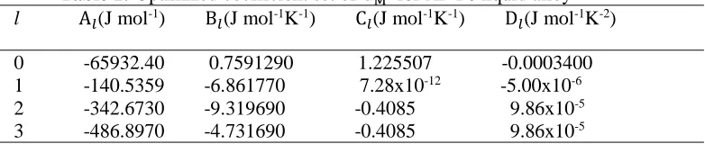
The optimized coefficients are obtained by the method of least square fitting using programming in computer software Microsoft Excel 2007 and are tabulated in the Table 1.
Table 1: Optimized coefficient set of GMXS for Al−Fe liquid alloy l A𝑙(J mol-1) B𝑙(J mol-1K-1) C𝑙(J mol-1K-1) D𝑙(J mol-1K-2)
0 -65932.40 0.7591290 1.225507 -0.0003400 1 -140.5359 -6.861770 7.28x10⁻¹² -5.00x10⁻⁶ 2 -342.6730 -9.319690 -0.4085 9.86x10⁻⁵ 3 -486.8970 -4.731690 -0.4085 9.86x10⁻⁵
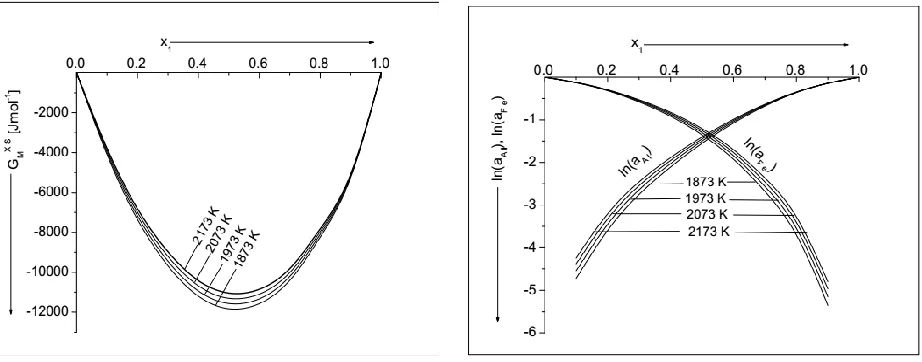
The compositional dependence of excess free energy of mixing at different temperatures computed from Equation (14a) using the values in table 1 are plotted in Figure 1. It can be observed that GMXS gradually decreases at elevated temperatures. It can, therefore, be forecasted that the complex formation tendency of the liquid alloy is the maximum at its melting temperature and gradually decreases at elevated temperatures.
Once the partial excess free energies of A and B are obtained, the activity coefficients at different temperatures are computed using the relation GpXS= RT ∑ ln γp, where the terms carry their usual
meanings. The compositional dependence of the activities of A (aAl) and B (aFe) are then computed from
Equation (5) and are plotted in Figure 2. It can be observed that the activities of the free monomers gradually increase with increase in the temperature of the alloy predicting the similar tendency as by GM
above. Similar results are predicted and explained by other researches [17, 23−25] for different alloy systems employing different techniques.
3.2 Structural Properties
The tendency towards complex formation and the local arrangements of atoms in the initial melt of the liquid systems can be further analyzed in terms of SCC(0), α1 and DM/Did. At a temperature and a
between the unlike atoms of the form A−B called ordering. Additionally, at such conditions if SCC(0) >
SCCid(0) for which α1> 0 and DM/Did< 1, then the association between the like atoms of form A−A or
B−B is favoured in the melt called segregating.
Fig. 1: Excess free energy of mixing (GMXS) as a
function of concentration of Al (x1) for Al−Fe
liquid alloy at different temperatures.
Fig. 2: Activities of Al (ln(aAl)) and Fe
(ln(aFe)) as a function of concentration of Al
(x1) for Al−Fe liquid alloy at different
temperatures.
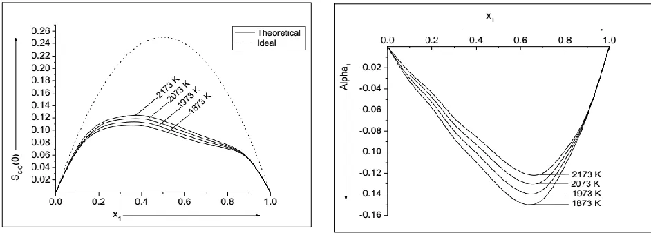
Figure 3 shows the compositional dependence of SCC(0) for the alloy at different temperatures computed
from Equation (9) with the aid of above determined model parameters. The predicted theoretical values of
SCC(0) gradually increases and get closure to their corresponding ideal values at elevated temperatures.
The deviation between the ideal and theoretical values of SCC(0) at complex formation concentration
(xCC= x1= 0.75) are 0.1121, 0.1093, 0.1065 and 0.1038 at temperatures 1873 K, 1973 K, 2073 K and
2173 K respectively forecasting that the tendency towards the complex formation is the most at 1873 K which is its melting temperature and the least at 2173 K. Theoretical investigations thus predict that the preferred system is the most interacting at 1873 K and the least at 2173 K.
The compositional dependence of α1 and DM/Did at different temperatures are computed from Equations
(10) and (11) and are portrayed in Figure 4. It can be observed that the plots of α1 gradually shallows with
increase in the temperature of the alloy predicting the decrease in the compound forming tendency at elevated temperatures. The computed values of α1 at compound forming concentration are 0.1298,
-0.1228, -0.1164 and -0.1103 at 1873 K, 1973 K, 2073 K and 2173 K respectively. The perusal of Figure 5 indicates that computed values of DM/Did gradually decreases at higher temperatures indicating the
similar results as discussed above.
3.3 Surface properties
f = 1.06 [14, 15, 23]. The molar volume (Vi0) of the pure component is estimated from the ratio of its atomic mass to density (m/ρ). The densities and the surface tension (σi0) of the pure components of the liquid alloy are taken from Table 2.
Fig. 3: The computed values of SCC(0) versus
concentration of Al (x1) for Al−Fe liquid alloy
at different temperatures.
Fig. 4: The computed values of α1 versus
concentration of Al (x1) for Al−Fe liquid alloy
at different temperatures.
Table 2: densities and surface tensions of pure metals [26] Metal Melting temp. Density Surface tension T0(K) ρ(kg m-3) σi0(N m-1)
Al 933 2385-0.280(T-T0) 0.914-0.35x10⁻³(T-T0)
Fe 1809 7015-0.880(T-T0) 1.872-0.49x10⁻³(T-T0)
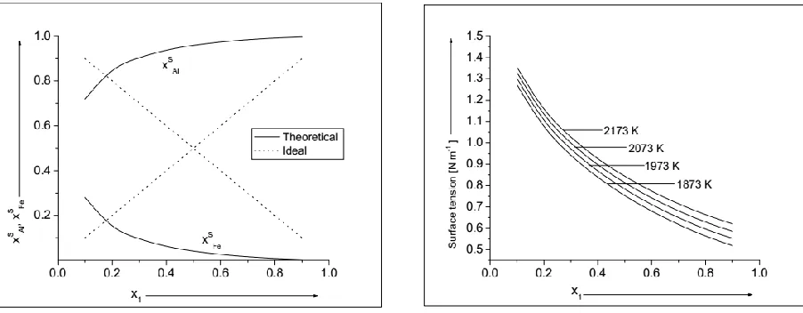
The computed values of σ as a function of concentration for Al−Fe liquid alloy at 1873 K are plotted in Figure 6. It can be observed that the theoretical value of σ is less than its ideal value at all concentrations. The perusal of Figure 7 communicates that the surface concentration of Al (xAlS ) is greater whereas that of
Fe (xFeS ) is less than their corresponding ideal values revealing that Al atoms segregates on the surface region and Fe atoms remains in the bulk region of the liquid mixture at 1873 K.
It has been already mentioned that the thermodynamic properties have been correlated with the Renovated Butler model to predict the surface properties of the preferred liquid alloys at different temperatures. The compositional dependence of σ, xAlS and xFeS are computed at afore mentioned temperatures from Equation
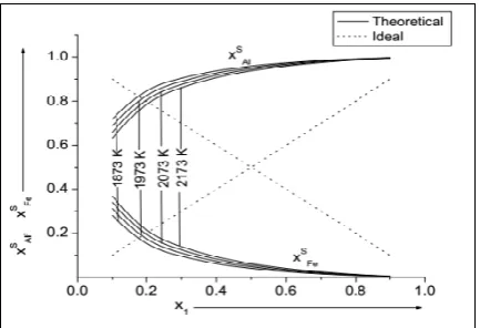
Figure 9 shows the compositional dependence of xAlS and xFeS for the alloy at different temperature. The computed values of xAlS gradually decreases whereas that of xFeS gradually increases with increase in the
temperatures of the melt above 1873 K. Both of these values get closure to their respective ideal values at
elevated temperatures. It can be thus predicted that the Al atoms move from surface region to the bulk region whereas the Fe atoms move from bulk region to the surface region with increase in temperature of the alloy to maintain equilibrium in the liquid phase.
Fig. 5: The computed values of DM/Did) versus
concentration of Al (x1) for Al−Fe liquid alloy
at different temperatures.
Figure 6: Surface tension (σ) versus concentration of Al (x1) for Al−Fe liquid alloy
at 1873 K.
Fig. 7: The computed values of surface concentration of Al (xAlS ) and Fe (xFeS ) versus
concentration of Al (x1) for Al−Fe liquid alloy
at 1873 K.
Fig. 8: The computed values of surface tension (σ) versus concentration of Al (x1) for Al−Fe
Fig. 9: The computed values of xAlS and xFeS versus concentration of Al (x1) for Al−Fe liquid alloy at
different temperatures.
4. Conclusions
The theoretical investigations forecast that the compound forming tendency of the preferred liquid alloy gradually decreases at higher temperatures. The alloy is found to be the most reactive at its melting temperature and this nature gradually declines at elevated temperature. The surface concentrations of Al decreases whereas that of Fe increases with increase in temperature of the alloy indicating the movement of former atoms from the surface to bulk region and that of later atoms from bulk to surface region. Additionally, the system shows ideal behaviour at higher temperatures.
References
[1] A.B. Bhatia, W.H. Hargrove, Concentration fluctuations and thermodynamic properties of some compound forming binary molten systems, Phys. Rev. B 10 (1974) 3186.
doi.org/10.1103/PhysRevB.10.3186.
[2] N.H. March, J.A. Alonso, Non-monotonic behaviour with concentration of the surface tension of certain binary liquid alloys, Phys. Chem. Liq. 46 (2008) 522. doi.org/10.1080/00319100801930466.
[3] R. Novakovic, Thermodynamics, surface properties and microscopic functions of liquid Al–Nb and Nb– Ti alloys, J. Non-Cryst. Solids, 356 (2010) 1593. doi.org/10.1016/j.jnoncrysol.2010.05.055.
[4] P.J. Flory, Thermodynamics of High Polymer Solutions, J. Chem. Phys. 10 (1942) 51. doi.org/10.10631/1.1723621.
[5] D. Adhikari, I.S. Jha, B.P. Singh, Structural asymmetry in liquid Fe–Si alloys, Phil. Mag. 90 (2010) 2687. doi.org/10.1080/14786431003745302.
[6] K. Hoshino, W.H. Young, On the electrical resistivity of the liquid Li-Pb alloy, J. Phys. F: Metal Phys. 10 (1980) 1365.doi.org/10.1088/0305-4608/10/7/003.
[7] S.K. Yadav, L.N. Jha, D. Adhikari, Thermodynamic and structural properties of Bi-based liquid alloys
Physica B, 475 (2015) 40. doi.org/10.1016/j.physb.2015.06.015.
[8] H. Ruppersberg, H.J. Reiter, A simple local pseudopotential for lithium, J. Phys. F: Metal Phys. 12 (1982) 1311. doi.org/10.10888/0305-4608/12/7/005.
[9] S.K. Yadav, L.N. Jha, D. Adhikari, Thermodynamic, structural, transport and surface properties of Pb-Tl
liquid alloy, Bibechana 13 (2016) 100. doi.org/10.3126/bibechana.v13i0.13443.
[10] A.S. Jordan, Metall. Trans. 1 (1970) 239.
[11] S. Lele, P. Ramchandrarao, Estimation of complex concentration in a regular associated solution
[12] I.S. Jha, D. Adhikari, B.P. Singh, Mixing behaviour of sodium-based liquid alloys, Phys. Chem. Liq., 50 (2012) 199. doi.org/10.1080/00319104.2011.569887.
[13] G. Kaptay, Partial Surface Tension of Components of a Solution, Langmuir 31 (2015) 5796. doi.org/10.1021/acs.langmuir.5b00217.
[14] G. Kaptay, Modelling equilibrium grain boundary segregation, grain boundary energy and grain boundary segregation transition by the extended Butler equation, J. Mater. Sci., 51 (2016) 1738. doi.org/10.1007/s10853-015-9533-8.
[15] S.K. Yadav, L.N. Jha, I.S. Jha, B.P. Singh, R.P. Koirala, D. Adhikari, Prediction of thermodynamic and surface properties of Pb−Hg liquid alloys at different temperatures, Phil. Mag. 96 (2016) 1909. doi.org/10.1080/14786435.2016.1181281.
[16] O. Redlich, A. Kister, Thermodynamics of Nonelectrolyte Solutions - x-y-t relations in a Binary System, Indust. Eng. Chem. 40 (1948) 345. doi.org/10.1021/ie50458a035.
[17] R.N. Singh, F. Sommer, Segregation and immiscibility in liquid binary alloys, Rep. Prog. Phys. 60 (1997) 57. doi.org/10.1088/0034-4885/60/1/003.
[18] D. Adhikari, S.K. Yadav, L.N. Jha, Thermo-physical properties of Al–Fe melt, J. Chin. Adv. Mater. Soc. 2 (2014) 149. doi.org/10.1080/22243682.2014.928603.
[19] P. Desai,Thermodynamic Properties of Selected Binary Aluminum Alloy Systems, J. Phys. Chem. Ref. Data, 16 (1987) 112.doi.org/10.1063/1.555788.
[20] I. Prigonine, R. Defay, Chem. Thermodynamics, Longmans Green and Co., London, 1974. [21] J.M. Cowley, An Approximate Theory of Order in Alloys, Phys. Rev. 77 (1950) 669.
doi.org/10.1103/PhysRev.77.669.
[2 2] L.S. Darken, R.W. Gurry, Phys. Chem. Metals, McGraw Hill, New York (1953).
[23] S.K. Yadav, L.N. Jha, D. Adhikari, Theoretical Modeling to Predict the Thermodynamic, Structural, Surface and Transport Properties of the Liquid Tl−Na Alloys at different Temperatures, J.N.P.S., 4 (2017) 101.
[24] O.E. Awe, Y.A. Odusote, L.A. Hussain, O. Akinlade, Temperature dependence of thermodynamic
properties of Si–Ti binary liquid alloys, Therm. Acta, 519 (2011) 1. doi.org/10.1016/j.tca.2011.02.028.
[25] G. Kaptay, On the Tendency of Solutions to Tend Toward Ideal Solutions at High Temperatures
Metall. Mater. Trans. A, 43 (2012) 531. doi.org/10.1007/s11661-011-0902-x.