Journal of Hydraulic Structures J. Hydraul. Struct., 2016; 2(1):34-47 DOI: 10.22055/jhs.2016.12649
Shape Optimization of an abrupt contraction using numerical
streamlining
Reza Yousefian1
Seyed Fazlolah Saghravani2
Abstract
This research was conducted to find a reliable technique to shape an abrupt contraction for minimizing the energy loss. The method may find broader applications in design of variety of transitional cross-sections in hydraulic structures. The streamlines in a 2-D contraction were calculated through solving the potential flow equations in rectangular and curvilinear coordinates. The natural cubic spline equations were applied to approximate the shape of streamlines. The streamlines close to the solid boundary, usually those that represent 5 and 95 percent of the discharge, were repeatedly mapped onto the solid boundary in a trial and error procedure until a negligible difference between two consecutive shapes was achieved. This procedure was applied through a code developed in C++, namely Streamlining Program Code or SPC. The initial and final shapes were used to validate SPC by the help of a robust CFD software, OpenFOAM. In a 2-D contraction with contraction ratio of 5, entrance velocity of 1 m/s and outlet pressure of atmosphere (P = 0 pa), the maximum spatial difference between the stream lines found by the code and OpenFOAM was limited to 2.74% that occurred in the entrance of the contraction. Finally, according to the validation, the streamlining technique and the code could successfully applied to shape optimization of hydraulic structures.
Keywords: hydraulic design; numerical technique; streamlining; grid generator; verification; OpenFOAM.
Received: 14 January 2016; Accepted: 27 June 2016
1. Introduction
In the recent decades, with the advancement of computational technology, the use of robust numerical methods to solve the complex equations of fluid mechanics became more feasible. The streamlined based design is a design philosophy to form the solid bodies so that offers the
1 Department of Civil Engineering, Shahrood University of Technology, Shahrood, Iran,
[email protected], Tel.: +98-23-32300259; fax: +98-23-32300259. (Corresponding author)
least resistance to fluid flow. Since the available new literature on details of streamlining techniques is limited, more research in this area seems to be useful.
The area of streamlined design has received great attention within different fields of application. Prior to 1960s, axial compressor and turbine design were based on streamlining, relied considerably on correlations of experimental data. Analytical research began to have greater impacts on this largely practical design approach towards the end of the 1950s. Since early 1960s, modern turbo-machinery design has mostly relied on CFD to develop three-dimensional blade sections. Nowadays, simple methods accompanied by empirical input are used for the mean-line design and flow modelling. These calculations are often left to the experienced designers who utilize CFD tools to reach to a good design [1]. In 2003, research on stationary fluid-structure interaction (FSI) problems was implemented for the sake of analysis and shape optimization of strongly coupled FSI systems by general, efficient and gradient based methods [2]. An optimized design for streamlining an intake of a small-scale turbojet engine carried out by Amirante et al. in 2007 [3]. In 2009, the streamlining procedure was used to design an inlet guide vane system of a mini hydraulic bulb-turbine, 3-stage axial-flow compressor and axial-flow hydraulic turbine [4] [5] [6]. Similarly, streamlining was applied to design and develop clamping and mold ejection systems to use in gravity die-casting machine and in optimization of bridge piers cross-section [7] [8].
This paper presents a numerical technique for streamlining of transitional cross-sections in hydraulic structures that carry incompressible-irrotational flow. This method is capable of streamlining cross-sections with positional constraints as well as considering the upstream characteristics in streamlining procedure. Note that, as streamlining leads transitional flows to be irrotational, assumption of irrotationality does not limit the applications of this streamlining technique. In this approach, first, the potential flow equations could be solved by any desired numerical method to obtain the streamlines, which the finite difference method (FDM) was used here for the sake of simplicity and attracting to a broad range of readers. Then, a streamline would be selected and mapped on the solid boundary to form a new curved boundary. Thereafter, accompanied by generating structured grids, the problem would be solved through iterative scheme for calculating the new streamlines. This iterative procedure continues until the differences between the coordinates of previous and current solid boundaries become less than the allowed tolerance. Eventually, a problem was adapted and solved to verify the applied technique by modelling obtained geometries in OpenFOAM.
2. Governing equations
This technique aimed to shape the cross-sections in reference to the streamlines coordinates, and thus, it needs to solve a stream function that is the description of the flow. The stream function satisfies the law of conservation of mass for incompressible, two-dimensional flows. According to the mass conservation law, the continuity equation can be written as equation Error! Reference source not found..
−1 𝜌
𝐷𝜌 𝐷𝑡 =
𝜕𝑢𝑖
𝜕𝑥𝑖 (1)
The density of fluid does not change appreciably along the fluid path under certain conditions according to the Boussinesq approximation. The conditions hold in most liquid flows and in the flows of gases where the speeds are less than about 100 m⁄s [9].
equation. In the case of irrotational flow, by substituting the definitions of stream function into the equation of vorticity, the so called Laplas Equation of stream function, the main differential equation for streamlining techniques, would be derived as Equation (2) [10].
𝛻2𝜓 =𝜕
2𝜓
𝜕𝑥2 + 𝜕2𝜓
𝜕𝑦2 = 0 (2)
3. Solving governing partial differential equation (PDE)
In order to solve the governing PDE, FDM was selected as approximations convert the partial derivatives to finite difference expression. As equation Error! Reference source not found. is an elliptic equation, point successive over-relaxation method (PSOR) was chosen for solution algorithm. In this algorithm, finite difference equations are solved at grid points. Therefore, first, grid points within the domain as well as the boundaries coordinates must be specified and then solving the PDE as algebraic equation is accomplished by finite difference formulations.
As the domains are categorized into two grid systems, structured and unstructured grids, the grid system of this technique was considered as structured with rectangular and nonrectangular physical domains [10].
3.1. Solving governing PDE within rectangular domain.
In the first stage, the domain is assumed as rectangular and grid points are specified as coincident with the boundaries of physical domain, thus the grid generation will be considerably simple. Therefore, the initial streamlines are obtained by utilizing PSOR method for solving the stream function equation. In this method, a second-order central differencing is used for the representation of the PDE. Thus, model Equation Error! Reference source not found. is approximated as follows.
ψi,jk+1= (1 − ω)ψi,jk + ω
2(1 + β2)[ψi+1,jk + ψi−1,jk+1 + β2(ψi,j+1k + ψi,j−1k+1)] (3)
In this equation, β is the ratio of step-sizes defined as β = Δx Δy⁄ . The variable ψ is solved at each grid point by using initial guessed values or previously computed values. Thus, k is defined as iteration level and since PSOR uses a trend to accelerate the solution procedure, the relaxation parameter ω which is necessary to be 0 < ω < 2 utilized in equation Error! Reference source not found. [10]. Thereafter, one of the streamlines in the rectangular domain is picked to map on the solid boundaries for creating the problem with new boundaries that will be solved in the next stage.
3.2. Solving governing PDE within nonrectangular domain
normal to the surface. Therefore, for transforming the physical space, first transformation of the governing PDE equation is accomplished, and then the grid would be generated by partial differential methods [10].
3.2.1. Transformation of the governing PDE
By defining the following relations between the physical and computational spaces, the chain rule is used for transforming the partial differentiation expressions.
𝜉 ≡ 𝜉(𝑥, 𝑦), 𝜂 ≡ 𝜂(𝑥, 𝑦) (4)
𝜕 𝜕𝑥= 𝜕𝜉 𝜕𝑥 𝜕 𝜕𝜉+ 𝜕𝜂 𝜕𝑥 𝜕 𝜕𝜂, 𝜕 𝜕𝑦= 𝜕𝜉 𝜕𝑦 𝜕 𝜕𝜉+ 𝜕𝜂 𝜕𝑦 𝜕 𝜕𝜂 (5)
Therefore, the model PDE (equation Error! Reference source not found.) would be transformed from physical space to computational space by applying equations Error! Reference source not found. as follows [11].
𝜕2𝜓 𝜕𝜉2[(
𝜕𝜉 𝜕𝑥) 2 + (𝜕𝜉 𝜕𝑦) 2 ] +𝜕 2𝜓
𝜕𝜂2[( 𝜕𝜂 𝜕𝑥) 2 + (𝜕𝜂 𝜕𝑦) 2
] + 2𝜕 2𝜓 𝜕𝜉𝜕𝜂[( 𝜕𝜂 𝜕𝑥) ( 𝜕𝜉 𝜕𝑥) + ( 𝜕𝜂 𝜕𝑦) ( 𝜕𝜉 𝜕𝑦)] +𝜕𝜓 𝜕𝜉(
𝜕2𝜉 𝜕𝑥2+
𝜕2𝜉 𝜕𝑦2) +
𝜕𝜓 𝜕𝜂(
𝜕2𝜂 𝜕𝑥2+
𝜕2𝜂 𝜕𝑦2) = 0
(1)
The transformed equation would be solved in the computational domain. In addition, it should be mentioned that the transformation derivatives (metrics) should be known in advance by using a numerical method to solve the metrics in the computational space. Generally, to solve the metrics with less complexity, Jacobian of transformation, J, is defined to formulate the metrics [10].
𝐽 = 1
(𝜕𝑥𝜕𝜉𝜕𝑦𝜕𝜂−𝜕𝑦𝜕𝜉𝜕𝑥𝜕𝜂) (2)
3.2.2. Gridgeneration
In this streamlining technique, the elliptic grid generators that work well in the domain with specified physical boundaries, were used as grid generator. For generating the grid with curved boundaries, the x and y coordinates of solid boundaries should be defined and thereafter a system of elliptic PDEs with the form of equations (4) is solved to determine the x and y coordinates of computational domain grid points in the physical space.
𝜕2𝜉 𝜕𝑥2+
𝜕2𝜉 𝜕𝑦2= 0,
𝜕2𝜂 𝜕𝑥2+
𝜕2𝜂
𝜕𝑦2= 0 (4)
Equation (4) would be solved by PSOR iterative technique mentioned in section 0. Because of computation of these PDEs takes place in computational rectangular domain with uniform grid spacing, the interchanging of the dependent variables (x, y) and independent variables (ξ, η) are required. For this purpose, the mathematical expressions should be employed to transform the elliptic PDEs to equations (5).
𝑎𝜕 2𝑥
𝜕𝜉2− 2𝑏 𝜕2𝑥 𝜕𝜉𝜕𝜂+ 𝑐
𝜕2𝑥 𝜕𝜂2= 0, 𝑎
𝜕2𝑦 𝜕𝜉2− 2𝑏
𝜕2𝑦 𝜕𝜉𝜕𝜂+ 𝑐
𝜕2𝑦
𝜕𝜂2 = 0 (5)
𝑎 = (𝜕𝑥 𝜕𝜂) 2 + (𝜕𝑦 𝜕𝜂) 2 , 𝑏 = (𝜕𝑥 𝜕𝜉) ( 𝜕𝑥 𝜕𝜂) + ( 𝜕𝑦 𝜕𝜉) ( 𝜕𝑦 𝜕𝜂) , 𝑐 = ( 𝜕𝑥 𝜕𝜉) 2 + (𝜕𝑦 𝜕𝜉) 2 (6)
After all, coordinates of the grid points in physical space (x, y) would be specified for the purpose of determining the metrics and ψ values in order to solve the governing PDE in nonrectangular domain [10].
4. Verification of the streamlining technique
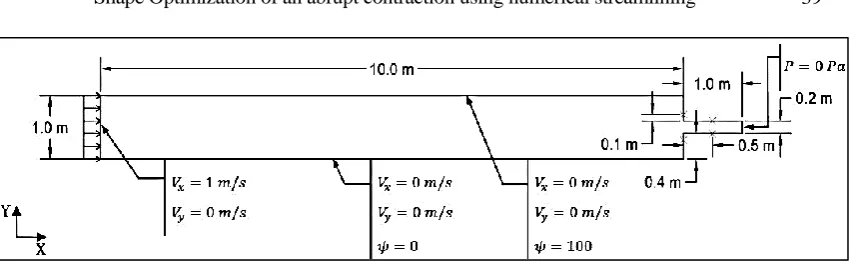
In order to verify the proposed streamlining technique, a 2D contraction problem for the sake of streamlining the entrance cross-section was chosen. The specifications of the problem was illustrated in Figure 1. In this problem, there were two pairs of positional constraints showed by cross markers in the entrance section to carry out streamlining in the boundaries between each pair of constraints. The fluid was assumed as water and the characteristics of boundaries and flow are as follows.
Inlet velocity in x-direction 1 m/s Inlet velocity in y-direction 0 m/s
Outlet pressure 0 Pa
Density of water 1000 kg/m3
Figure 1. Dimensions and boundary conditions of the problem
A streamlining programing code (SPC) based on details discussed in section 0, was written in C++ programming language by using the Microsoft Visual Studio Express edition 2013 as compiler. In this software, the standard libraries of C++ were used for calculations and the Fast Light Tool Kit 1.3.3 (FLTK) was utilized as Graphical User Interface (GUI) for illustrating the streamlines and streamlined cross-sections. Also, Open Source Field Operation and Manipulation (OpenFOAM) software with C++ library was employed to verify SPC. The version 2.2.2 of OpenFOAM was executed on Ubuntu12.04. In this application, the grid generated by blockMesh, potentialFoam used as solver and the version 3.12.0 of ParaView utilized for post-processing.
5. Results and discussions
The problem was solved by SPC and OpenFOAM software; by comparing the results of SPC and OpenFOAM software, the correctness of this numerical technique would be investigated in the following.
5.1. Results and solution algorithm of SPC
In order to streamline the contraction problem stated above, first the problem was solved in the rectangular domain, shown in Figure 1, by scheme discussed in section 0. The boundary conditions applied for this problem in SPC were shown in Figure 2. It should be noted that the boundary conditions of the stream function values in inlet and outlet were calculated based on mass conservation law. In this figure, is the node number in inlet and outlet sections.
The grid generated for the rectangular space had constant step-size in x and y direction and also the value of step-size was selected as 0.05 m and equaled to each other in both directions. Streamlines of this problem were obtained as a result of the first loop of streamlining, Figure 3.
Figure 3. Streamlines obtained in the first loop of streamlining in SPC
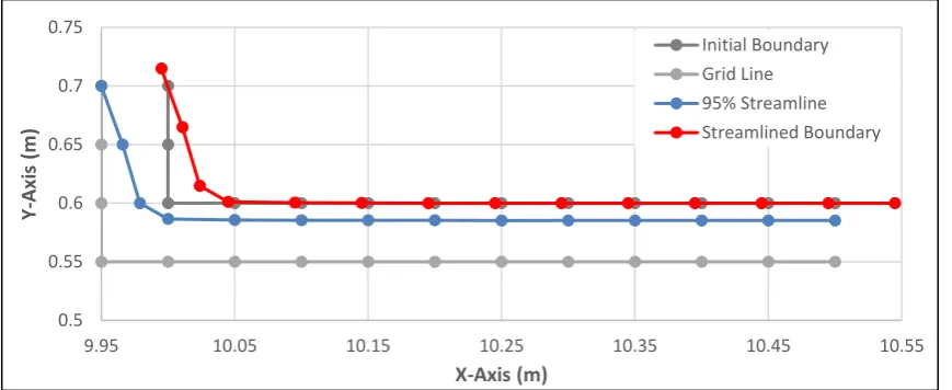
After obtaining streamlines in the rectangular domain, the streamline of ψ = 95% shown by blue line in Figure 4 selected to map on the solid boundary. For this purpose, by moving the selected streamline to the constraints mentioned in the problem, the new solid boundary, illustrated by red line in Figure 4, was formed.
Figure 4. Mapping a streamline on solid boundary
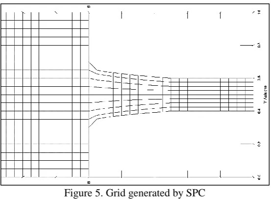
Therefore, the new problem with curved boundaries would be generated. This problem with nonrectangular domain was solved by the technique explained in section 0. Figure 5 illustrates the grid generated by SPC for this problem.
0 0.1 0.2 0.3 0.4 0.5 0.6 0.7 0.8 0.9 1
0 1 2 3 4 5 6 7 8 9 10 11
Y -A xi s (m ) X-Axis (m) ψ=0% ψ=10% ψ=20% ψ=30% ψ=40% ψ=50% ψ=60% ψ=70% ψ=80% ψ=90% ψ=100% 0.5 0.55 0.6 0.65 0.7 0.75
9.95 10.05 10.15 10.25 10.35 10.45 10.55
Figure 5. Grid generated by SPC
Finally, by defining the convergence criteria as the positional difference between selected streamline, here 95% streamline, and the previous streamlined boundary, this iterative procedure was carried out until the differences became less than 1.0E-11 m and then the streamlined section was obtained. Figure 6 illustrates the streamlined cross-section and streamlines calculated in this domain that as the grid points in the target area increased, the shape would be smoother.
Figure 6. Streamlined cross-section and streamlines in curved boundary domain obtained from SPC
5.2. OpenFOAM properties and results
For modelling the problem to verify SPC, two problems with rectangular and nonrectangular spaces, illustrated in Figure 3 and Figure 6, were modelled in OpenFOAM. Velocities and pressures conditions of boundaries assigned to the models are shown on Figure 7. Noted that the boundary conditions of both models were the same.
0 0.1 0.2 0.3 0.4 0.5 0.6 0.7 0.8 0.9 1
0 1 2 3 4 5 6 7 8 9 10 11
Y
-A
xi
s
(m
)
X-Axis (m)
Figure 7. Boundary conditions of models in OpenFOAM
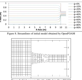
By modelling the problem in OpenFOAM software, grid and stream function accuracy of SPC results were considered as criteria to verify the CFD code. Since there were two models discussed above with rectangular and nonrectangular domain, the cited criteria was studied in these two models. For illustration purposes, Figure 8 and Figure 10 show the streamlines obtained by OpenFOAM and Figure 9 illustrates the grid generated by blockMesh in OpenFOAM. Also these figures would be compared to Figure 3 , Figure 6 and Figure 5, the results of SPC, respectively.
Figure 8. Streamlines of initial model obtained by OpenFOAM
Figure 9. Grid generated by blockMesh in OpenFOAM 0
0.2 0.4 0.6 0.8 1
0 1 2 3 4 5 6 7 8 9 10 11
Y
-A
xi
s
(m
)
X-Axis (m)
Figure 10. Streamlines of streamlined model obtained by OpenFOAM
5.3. Results comparison
The nodes coordinates of OpenFOAM and SPC models were compared to each other in the following to verify the grids. In rectangular domain, the grids were the same as expected but some differences in grid points coordinates of nonrectangular domain were observed. The maximum positional difference of grid points generated by blockMesh in OpenFOAM and SPC was 0.018 m in x-direction. Figure 11 illustrates the position of maximum differences in the domain.
Figure 11. Position of maximum differences between x-coordinate of grids
The differences in y-direction are as shown in Figure 12. The maximum difference between corresponding nodes was 0.014 m.
Figure 12. Position of maximum differences between y-coordinate of grids 0
0.2 0.4 0.6 0.8 1
0 1 2 3 4 5 6 7 8 9 10 11
Y
-A
xi
s
(m
)
X-Axis (m)
ψ=0%
ψ=10%
ψ=20%
ψ=30%
Since the differences in the domain were in a small part of the domain, Figure 13 and Figure 14 were prepared to show more precise place of differences.
Figure 13. Magnified position of maximum differences between x-coordinate of grids
Figure 14. Magnified position of maximum differences between y-coordinate of grids
Although differences existed in grids generated by OpenFOAM and SPC were less than 5% but unchanging x-coordinate of grids in SPC, differences in approximation methods and schemes employed in these models are accounted for these displacements.
For considering the values of stream function in both models by OpenFOAM, the non-dimensional stream function values of grid points in physical domain (with the same coordinates) were calculated and compared to each other. As shown in Figure 8, the maximum difference between stream function values in rectangular domain models was 1.3E -4%. Since the grids of both OpenFOAM and SPC were the same, the value was expected.
Figure 15. Position of maximum differences between ψ values
Figure 16 illustrates more details of differences showed in Figure 15 to compare the stream function results.
Figure 16. Magnified position of maximum differences between ψ values
The following issues could cause some inconsistencies observed in the stream function values. As OpenFOAM solves the PDEs by finite volume method (FVM), approximations used in this application differ from SPC, which utilizes FDM. In addition, solution schemes and numerical technique employed by these CFD tools make some differences in results of modelling. Moreover, by considering the positions of differences in grids of models, Figure 13 and Figure 14, and position of maximum differences of stream function values shown in Figure 16, the differences in stream function values would be expected. Therefore, according to these reasons include differences in grid points coordinates and also the methods employed for modelling in these CFD tools, the maximum difference of stream function value was accepted as allowable value for verification.
6. Conclusions
of upstream flow and positional constraints on the shape of cross-sections in order to study the numerical aspects of streamlining in this application field. For this purpose, the grid generation technique, methods of solving rectangular and nonrectangular domains for streamlining in SPC were investigated with the help of OpenFOAM software. Comparison of stream function values and those from the modelling of both types of domains in OpenFOAM illustrated that the grid generation technique plays an important role in accuracy and correctness of numerical results. In the case of rectangular domain, FVM and FDM provide almost identical answer to the problem, while for nonrectangular domain some differences are observed. The results of comparing the nonrectangular grids demonstrated that although a problem can be solved within a one directional grid, for the sake of accuracy, the grid should be generated in all directions of the problem. Furthermore, as many problems in numerical methods are divided to some blocks that are rectangular or nonrectangular, for grid generation procedure, all blocks of the problem should be considered as a unit block until the sudden change in the grid does not affect the results. Finally, modelling grids and both types of domain in OpenFOAM showed that in general, there was a good agreement between the results of SPC and OpenFOAM. Therefore, the numerical technique employed in SPC to streamline different transitional sections is verified and capable to improve the other streamlining techniques.
7. Acknowledgements
The authors would like to thank Dr. A. A. Pouyan and Ms. Z. Elmi for their assistance in the course of this research.
References
1. J. H. Herlock and J. D. Denton, "A review of some early design practice using computational fluid dynamics and a current perspective," Journal of Turbomachinery,
vol. 127, pp. 5-13, January 2005.
2. E. Lund, H. Moller and L. A. Jakobsen, "Shape design optimization of stationary fluid-structure interaction problems with larg displacements and turbulence," Structural and Multidisciplinary Optimization, vol. 25, pp. 283-392, 2003.
3. R. Amirante, L. A. Catalano, A. Dadone and V. S. E. Daloiso, "Design optimization of the intake of a small-scale turbojet engine," Computer Modeling in Engineering and Sciences, vol. 18, pp. 17-30, 2007.
4. L. M. Ferro, L. M. Gato and A. F. Falcao, "Design and experimental validation of the inlet guide vane system of a mini hydraulic bulb-turbine," Renewable Energy, vol. 35, pp. 1920-1928, 2009.
5. J. Takachi Tomita and J. R. Barbosa, "The use and comparison of avialabe design tools for a 3-stage axial-flow compressor: meanline, streamline curvature and cfd," in 20th International congress of mechanical engineering, Gramado, 2009.
7. V. Sharma and O. PrakashShukla, "Design and development of clamping and ejection systems for mould used on gravity die casting machine," International Journal of Engineering and Technology, vol. 2, no. 10, pp. 890-897, 2013.
8. L. Junhong and T. Junliang, "Streamlining of bridge piers as scour countermeasures: optimization of cross section," in Transport Research Board 94th Annual Meeting, Washington, 2015.
9. K. P. Kundu and I. M. Cohen, Fluid mechanics, 4th ed., Burlington, Massachusetts: Academic Press, 2010.
10. K. K. Hoffmann and S. T. Chiang, Computaional fluid dynamics, 4th ed., vol. 1, Wichita, Kansas: Engineering Education System, 2000.