Please cite this article as: H. Bazoobandi, Wavelet Neural Network with Random Wavelet Function Parameters, International Journal of Engineering (IJE), TRANSACTIONS A: Basics Vol. 30, No. 10, (October 2017) 1510-1516
International Journal of Engineering
J o u r n a l H o m e p a g e : w w w . i j e . i rWavelet Neural Network with Random Wavelet Function Parameters
H. Bazoobandi*
Department of Computer Engineering, Esfarayen University of Technology, Esfarayen, North Khorasan, Iran
P A P E R I N F O
Paper history:
Received 08 November 2016
Received in revised form 08 August 2017 Accepted 08 September 2017
Keywords:
Wavelet Neural Network Training Algorithm Moore-Penrose Inverse Random Parameter Values
A B S T R A C T
The training algorithm of Wavelet Neural Networks (WNN) is a bottleneck which impacts on the accuracy of the final WNN model. Several methods have been proposed for training the WNNs. From the perspective of our research, most of these algorithms are iterative and need to adjust all the parameters of WNN. This paper proposes a one-step learning method which changes the weights between hidden layer and output layer of the network; meanwhile, the wavelet function parameters are randomly assigned and kept fixed during the training process. Besides the simplicity and speed of the proposed one-step algorithm, the experimental results verify the performance of the proposed method in terms of final model accuracy and computational time.
doi: 10.5829/ije.2017.30.10a.12
1. INTRODUCTION1
Recently, Wavelet Neural Networks (WNNs) have been used in different areas of science, e.g. engineering applications, to find more competitive final models in comparison to the conventional Neural Networks (NNs). Sigmoidal activation function in Feed-forward Neural Networks (FNNs) are replaced with wavelet functions in WNNs [1]. Wavelet functions have interesting properties, including time-frequency localization and multi-resolution [2]. These properties lead to exciting applications for wavelets [3], and make WNNs more successful than FNNs [2].
Feedforward WNN is introduced by Zhang, and Benvensti in [4] to be a wavelet function employed as an activation function in WNN [4] instead of Sigmoid in NNs. They have also presented theoretical analysis to demonstrate universal approximation property of WNN. Among the considerable issuses regarding WNNs is the training algorithms. There are two types of parameters needing to be adjusted during training: 1) biases and weights, as conventional NNs, and 2)wavelet function parameters (including translation and dilation parameters). Nevertheless, there are numerous studies on training WNNs.
*Corresponding Author’s Email: [email protected] (H. Bazoobandi)
algorithm. In the first phase, i.e. the initialization phase, a GA hase been applied with the aim to find out suitable initial values for all of the parameters. Next, a Backpropagation learning based on chain rule of differentiation has been employed to adjust the wavelet functions and weight parameters. Another similar hybrid method is proposed [12] which in all the parameters of fuzzy WNN are initiated using Particle Swarm Optimization (PSO) and then a gradient descent algorithm is applied to find accurate values of these parameters [12]. The most remarkable deficiency in using EAs in this context is its high computational complexity, whereas achieving a higher accuracy is the most outstanding efficiency of using EAs compared to classical method.
Neural Network with Random Weights (NNRWs) is another topic related to the present research. The idea of NNRWs originates from a study by Schmidt, et al. [13] on single hidden layer network, where the input weights and biases are assigned randomly, and the output weights are calculated via solving a linear least square problem in just a single step [13]. Unfortunately, the method could not guarantee universal approximation ability. Another related research is the Random Vector Functional Link (RVFL) network, proposed by Pao and Takefuji [14] and Pao et al. [15] which further developed [16-18]; the method is named Extreme Learning Machine (ELM) in more recent studies [19]. Input weights and biases are generated randomly in RVFL, and output weights are calculated using pseudoinverse of the hidden output matrix. The theoretical justification for universal approximation ability of RVFL is demonstrated by Igelnik and Pao [16]. A comprehensive review on random NNs are given by Li and Wang [20] and Zhang and Suganthan [21]. Random NNs are high-speed in training due to their lower number of parameters to be adjusted.
Most of the previously-introduced training methods for WNNs have two important features from the perspective of the present research: I) the iterative structure for training methods, and II) the fact that all of the parameters need to be adjusted during the training phase. Zainuddin and Pauline proposed an iterative method in which the wavelet function parameters are initialized and do not change during the training process, but weights between the hidden layer and the output layer of WNN are adjusted [22]. The study shows the dependency parameters in WNNs, so that desirable weights can be obtained for any reasonable values for wavelet function parameters [22].
The present paper aimed to propose a one-step training algorithm for WNNs, which adjusts only the output weights in just one step. Wavelet function parameters, biases, and input layer weights were randomly assigned here. The proposed method also integrated the WNNs approximation ability and the high
speed training of random neural networks. The rest of the paper is organized as follows. The structure of WNNs is briefly introduced in Section 2. The proposed method is presented in Section 3. Experimental results verify the performance of the proposed method in Section 4. Finally, the concluding remarks are provided in Section 5.
2. WAVELET NEURAL NETWORK
Wavelet Neural Network (WNN) is introduced by Zhang, and Benveniste [4]. Wavelet functions have been used as activation function in WNNs instead of conventional Sigmoid function in FNNs. The output of WNN can be described as follows:
1
( ),
L
j i i
i i
x t
Y w
d
(1)where
w
i stands for the weight between ith hidden node(i=1…L) and the output node, and the function
(.)
describes the activation function output. ti, and di are the translation and dilation of the wavelet in ith hidden node, respectively. xj is the jth input sample (j=1..N). Mexican Hat wavelet function is used in this study, the output of which could be calculated as follows:
1 2 x2
( x ) ( 1 2 x ) exp( ).
2 d
(2)
3. PROPOSED ONE-STEP TRAINING METHOD
In this section, a one-step method is proposed for training the WNNs. The idea of our proposed method comes from the concept of random algorithms for training NNs, e.g. [13, 15]. In this type of algorithms, input weights and biases are assigned randomly, and the output weights of the NN are calculated using pseudeinverse of the hidden output matrix.
For training the WNNs, there are two types of parameters in Equation (1) which need to be adjusted: Wavelet function parameters (t, d), and the weights and biases of network (w, b). In our proposed method, wavelet function parameters were chosen randomly using the uniform distribution in a range which depends on training sample values. Then, the Equation (1) can be represented as Y W , where W[w w1, 2,....,wL] and
1 1 1 1
1 1
( , , ) . . . ( , , )
. .
. .
. .
( , , ) . . . ( , , ) T L L
N N L L
x t d x t d
x t d x t d
The
matrix can be calculated easily, because the wavelet function parameters are not changed during the training process. The optimum values of w (w*), leads to W* T, where T is the output vector for N training samples [ , ,...,1 2 ]TN
T t t t .
In most of the situations, is not full column rank or even ill-conditioned. Therefore, the weights (w) can be obtained using Moore-Penrose generalized inverse of the through solving the following criterion:
2 2 * { }, min N w R T w W
(3)where, the least square solution is W* †T. † shows the Moore-Penrose generalized inverse where
† 1
( T ) T
.
According to the discussion in the previous paragraphs, the proposed method can be summarized as follows:
Randomly assign wavelet function parameters (t,
d), input weights, and biases.
Calculate the matrix .
Calculate the pseudoinverse matrix †.
Calculate the output weights as W* †T.
The most remarkable advantage of the proposed method over the previously-introduced methods for training WNNs is its non-iterative process and a much less computation. Furthermore, by increasing the number of hidden neurons or the size of training set, the iterative-based methods converge more slowly [23]. Experimental results [23] show that random NNs, similar to our proposed method, demand more hidden neurons to achive the same accuracy as other networks. Therefore, being a more complex model can be the main deficiency of our poposed method. Wavelet functions in the hidden layer of the proposed network leads to a higher approximation ability in comparison with NNRW [13], and RVFL [14-18]. Experimental results in the next section confirmed the superior performance of the proposed method with respect to both WNN training methods and random neural networks.
4. EXPERIMENTAL RESULTS
4. 1. Simulation Examples Four well-known benchmark functions have been used from the literature in order to assess the performance of our proposed method.
In addition to our proposed method, FWNN-GA [8], SLFRWNN [7], NNRW [13], and RVFL [13] are implemented and used in comparisons. 50 hidden units used in the single hidden layer of the proposed method, NNRW, and RVFL (L=50). The parameters of
FWNN-GA, and SLFRWNN also set with similar values in the seminal papers [7, 8].
4. 1. 1. Approximation of a Piecewise Function
The piecewise function with the following situation has been used in the literature [4, 7-10]:
2.186 12.864, 10 2
1( ) 4.246 , 2 0 ,
10exp( 0.05 0.5)sin[(0.03 0.7) ], 0 10
x x
F x x x
x x x x
(4)
200 training samples uniformly distributed over [-10, 10] are generated. The following Performance Index (PI) [4, 7-10] were used to evaluate the performance of the models: 2 1 2 1 ( ) , ( ) N i i i N i i t y PI t t
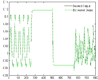
(5)where, ti and yi stand for the desired and the obtained outputs of the model, respectively. t represents the average of ti values. Table 1 compares the performance of the proposed method with the other approaches. The excellent ability of estimation of the proposed method can be observed in Table 1. It can be seen in Figure 1 that the output of the proposed model was very close to the desired output.
4. 1. 2. Dynamic System Identification Example1
The following system identification [6, 7, 12] was taken into account in this example:
2
2 ( ) 0.72 ( 1) 0.025 ( 2) ( 1) 0.01 ( 2) 0.2 ( 3),
F y k y k y k u k u k u k (6) where, y k( ) is the kth plant output; u k( ) is the excitation signal defined as follows:
ksin , k 250 25
250 k 500
1, 500 k 750
k 0.3 sin k / 25 0.1 sin k / 32 0.6 sin , 75 1,
0 k 1000. ) 10 u( k (7)
Root Mean Square Error (RMSE) given in Equation (8) was used as performance criterion:
K 2 i i 1 R y i MSE K t .
(8)4. 1. 3. Dynamic System Identification Example2
This example considers the following nonlinear dynamic plant:
F3y( k ) f(y(k-1),y(k-2),y(k-3),u(k),u(k-1)), (9)
where:
1 2 3 5 3 4
1 2 3 4, 5 2 2
3 2
x x x x ( x 1 ) x
f ( x , x , x ,
x x
1 x
x ) , (10)
y(k-i) in Equation (9) was the i-step delayed output of
the plant. u(k) and u(k-1) was the current and delayed inputs of the plant which can be calculated using Equation (7). RMSE in Equation (8) was used as performance criterion. As the previous example, 1000 training samples were generated with uniform random distribution in the interval [-1, 1]. Figure 3 shows the performance of the proposed method, and Table 3 compares the RMSE values with other methods in the literature.
TABLE 1. Comparison of simulation results of different
models for Approximation of a piecewise function (F1)
Model PI
Proposed WNN 0.0053
WN [4] 0.05057
SLFRWNN [7] 0.01901
FWNN-GA [8] 0.0303
WaveARX NN [9] 0.0480
Evolving WNNs [10] 0.0300
NNRW [13] 0.6166
RVFL [15] 0.0334
Figure 1. The comparison of outputs between the original
function and the proposed WNN for piecewise function (F1)
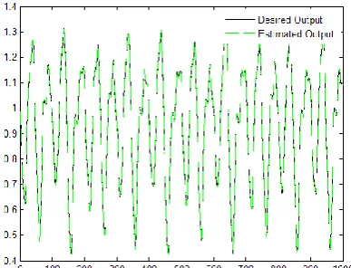
Figure 2. The comparison of outputs between the original
function and the proposed WNN for system identification example1 (F2)
Figure 3. The comparison of outputs between the original
function and the proposed WNN for system identification example 2 (F3)
TABLE 2. Comparison of simulation results of different
models for dynamic system identification example1 (F2)
Model RMSE
Proposed WNN 3.13209e-05
FWNN I [6] 0.019736
FWNN II [6] 0.018713
SLFRWNN [7] 0.0042
FWNN-GA [8] 0.0044
FWNN [12] 0.0067
NNRW [13] 6.7995e-04
TABLE 3. Comparison of simulation results of different models for dynamic system identification example2 (F3)
Model RMSE
Proposed WNN 0.0015
FWNN I [6] 0.029179
FWNN II [6] 0.028232
SLFRWNN [7] 0.023
FWNN-GA [8] 0.0369
FWNN [12] 0.0202
NNRW [13] 0.0104
RVFL [15] 0.0013
4. 1. 4. Mackey-Glass Time Series Prediction Mackey-Glass time series is one of the other benchmarks which have been used in the literature. It is defined as follows:
10
0.2x t
0.1x t , 1 x
(t
t
x )
(11)
where, =17, and x(0)=1.2. a dataset with 1000 samples is produced by the following form:
d
F 4{X x t 18 x t 12 x t 6 x t
d
y x(t6)}.
(12)
The estimation ability of the proposed method for Mackey-Glass time series data depicted in Figure 4. Comparison with the other methods based on RMSE measure are given in Table 4. It can be seen from the results (Table 4), that our proposed method attains a smaller error than others, except FWNN II [6].
4. 2. Wavelet Function Effect In this section of the paper, the effect of wavelet function type in the proposed method will be studied.
Figure 4. The comparison of outputs between the original
function and the proposed WNN for Mackey-Glass time series (F4)
TABLE 4. Comparison of simulation results of different
models for Mackey-Glass time series (F4)
Model RMSE
Proposed WNN 0.0054
FWNN I [6] 0.0257
FWNN II [6] 0.0035
SLFRWNN [7] 0.0068
FWNN-GA [8] 0.0292
NNRW [13] 0.0091
RVFL [15] 0.0102
RBF 0.0072
ANFIS 0.007
Backpropagation NN 0.02
Three well-known wavelet functions are taken into consideration here, i.e. Mexican-Hat, Gaussian, and Morlet. Table 5 shows the obtained RMSE for the benchmarks in the previous section. The results of Table 5 delineate that our proposed method using the Gaussian and Mexican-Hat wavelet function finds better solutions. Nevertheless, there were no significant differences regarding the accuracy of the models with different wavelet functions.
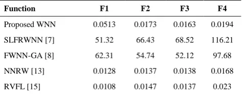
4. 3. Comparison of the Computational Time
Computational time for different methods are reported in this section. In simulations, all methods in Table 6
were implemented in MATLAB 8.4 (2014)
environment, running a Pentium Core2Duo processor with a speed of 2.00GHz and 2 GBytes of RAM. Table 6 shows the computational time for different methods in seconds. The proposed method, NNRW [13] and RVFL [15] are non-iterative algorithms, while the others, i.e. SLFRWNN [7] and FWNN-GA [8] are iterative methods. It can be observed in the results in Table 6 that non-iterative methods, as expected, need much lower computation times. Furthermoer, in the category of non-iterative methods, computation times were very close.
TABLE 5. The effect of wavelet function type on the
performance of the proposed method
Function Mexican-Hat Gaussian Morlet
F1 0.0053 (1) 0.0178(3) 0.0091(2)
F2 3.132e-5 (2) 2.925e-5 (1) 8.589e-5 (3)
F3 0.0015 (2) 0.00099 (1) 0.0039 (3)
F4 0.0054 (3) 0.0051 (2) 0.0046 (1)
Total Rank 8 (2) 7 (1) 9 (3)
TABLE 6. Comparison of computation time of algorithms (Sec.)
Function F1 F2 F3 F4
Proposed WNN 0.0513 0.0173 0.0163 0.0194
SLFRWNN [7] 51.32 66.43 68.52 116.21
FWNN-GA [8] 62.31 54.74 52.12 97.68
NNRW [13] 0.0128 0.0137 0.0138 0.0168
RVFL [15] 0.0108 0.0147 0.0137 0.023
5. CONCLUSION
This paper proposed a non-iterative parameter estimation method for training the wavelet neural network. A wavelet neural network has two types of parameters, namely wavelet function parameters (translation, dilation) and the weights between the hidden layer and output layer. In our proposed method, wavelet function parameters were initialized randomly and were kept fixed. Afterwards, Moore-Penrose generalized inverse of the output matrix of the model is calculated to obtain the precise values of weight parameters. The simple and fast proposed method outperformed the other methods even in terms of accuracy of the final model.
6. REFERENCES
1. Bazoobandi, H. and Eftekhari, M., "A differential evolution and spatial distribution based local search for training fuzzy wavelet neural network", International Journal of Engineering-Transactions B: Applications,Vol. 27, No. 8, (2014), 1185-1194.
2. Bazoobandi, H.-A. and Eftekhari, M., "A fuzzy based memetic algorithm for tuning fuzzy wavelet neural network parameters",
Journal of Intelligent & Fuzzy Systems,Vol. 29, No. 1,(2015), 241-252.
3. Daubechies, I., "Ten lectures on wavelets". SIAM, (1992). 4. Zhang, Q. and Benveniste, A., "Wavelet networks", IEEE
transactions on Neural Networks,Vol. 3, No. 6, (1992), 889-898.
5. Lin, C.-J., "Wavelet neural networks with a hybrid learning approach", Journal of Information Science and Engineering,Vol. 22, No. 6, (2006), 1367-1387.
6. Abiyev, R.H. and Kaynak, O., "Fuzzy wavelet neural networks for identification and control of dynamic plants—a novel structure and a comparative study", IEEE Transactions on Industrial Electronics,Vol. 55, No. 8,(2008), 3133-3140. 7. Ganjefar, S. and Tofighi, M., "Single-hidden-layer fuzzy
recurrent wavelet neural network: Applications to function approximation and system identification", Information Sciences,Vol. 294, (2015), 269-285.
8. Tzeng, S.-T., "Design of fuzzy wavelet neural networks using the GA approach for function approximation and system identification", Fuzzy Sets and Systems,Vol. 161, No. 19,
(2010), 2585-2596.
9. Chen, J. and Bruns, D.D., "WaveARX neural network development for system identification using a systematic design synthesis",Industrial & Engineering Chemistry Research,Vol. 34, No. 12, (1995), 4420-4435.
10. Yao, S., Wei, C., and He, Z., "Evolving wavelet neural networks for function approximation",Electronics Letters,Vol. 32, No. 4,
(1996), 360-369.
11. Hashemi, S.M.A., Haji Kazemi, H., and Karamodin, A., "Verification of an Evolutionary-based Wavelet Neural Network Model for Nonlinear Function Approximation", International Journal of Engineering-Transactions A: Basics,Vol. 28, No. 10, (2015), 1423-1429.
12. Cheng, R. and Bai, Y., "A novel approach to fuzzy wavelet neural network modeling and optimization", International Journal of Electrical Power & Energy Systems,Vol. 64, No. (2015), 671-678.
13. Schmidt, W.F., Kraaijveld, M.A., and Duin. R.P., "Feedforward neural networks with random weights", in Pattern Recognition, Vol. II. Conference B: Pattern Recognition Methodology and Systems, Proceedings., 11th IAPR International Conference on. IEEE, (1992).
14. Pao, Y.-H. and Takefuji, Y., "Functional-link net computing: theory, system architecture, and functionalities",Computer,Vol. 25, No. 5,(1992), 76-79.
15. Pao, Y.-H., Park, G.-H., and Sobajic, D.J., "Learning and generalization characteristics of the random vector functional-link net",Neurocomputing,Vol. 6 ,.No. 2,(1994), 163-180. 16. Igelnik, B. and Pao, Y.-H., "Stochastic choice of basis functions
in adaptive function approximation and the functional-link net",
IEEE transactions on Neural Networks,Vol. 6, No. 6,(1995), 1320-1329.
17. Mc Loone, S. and Irwin, G., "Improving neural network training solutions using regularisation",Neurocomputing,Vol. 37, No. 1, (2001), 71-90.
18. McLoone, S., Brown M.D., Irwin G., Lightbody A., "A hybrid linear/nonlinear training algorithm for feedforward neural networks",IEEE transactions on NeuralNetworks,Vol. 9, No. 4,(1998), 669-684.
19. Huang, G.-B., Zhu, Q.-Y., and Siew, C.-K., "Extreme learning machine: theory and applications", Neurocomputing,Vol. 70, No. 1,(2006), 489-501.
20. Li, M. and Wang, D., "Insights into randomized algorithms for neural networks: Practical issues and common pitfalls",
Information Sciences,Vol. 382, (2017), 170-178.
21. Zhang, L. and Suganthan, P.N., "A survey of randomized algorithms for training neural networks", Information Sciences,Vol. 364, (2016), 146-155.
22. Zainuddin, Z. and Pauline, O., "Modified wavelet neural network in function approximation and its application in prediction of time-series pollution data", Applied Soft Computing,Vol. 11, No. 8, (2011), 4866-4874.
Wavelet Neural Network with Random Wavelet Function Parameters
H. Bazoobandi
Department of Computer Engineering, Esfarayen University of Technology, Esfarayen, North Khorasan, Iran
P A P E R I N F O
Paper history:
Received 08 November 2016
Received in revised form 08 August 2017 Accepted 08 September 2017
Keywords:
Wavelet Neural Network Training Algorithm Moore-Penrose Inverse Random Parameter Values
ديكچ ه
یارب یفلتخم یاهشور نونکات .تسا ییاهن لدم تقد رب رثوم هاگولگ کجوم یزاف یبصع یاه هکبش رد شزومآ یاه متیروگلا
،ور شیپ قیقحت هاگدید زا .تسا هدش داهنشیپ کجوم یبصع یاه هکبش شزومآ دنتسه رارکت رب ینتبم اه متیروگلا نیا رتشیب
همه یتسیاب و نیب یاه نزو میظنت یارب یا هلحرم کت یشور هلاقم نیا رد .دنیامن میظنت ار کجوم یبصع هکبش یاهرتماراپ
ات و تسا هدش یهدرادقم یفداصت تروصب کجوم عبات یاهرتماراپ نینچمه .تسا هدش داهنشیپ یجورخ هیلا و یفخم هیلا
اس رب هولاع .تسا هدش هتفرگ رظن رد تباث شزومآ دنیارف نایاپ یبرجت جیاتن ،یا هلحرم کت یداهنشیپ شور تعرس و یگد