THE EFFECT OF COSMIONS ON THE STABILITY OF MAIN SEQUENCE
STELLAR CORES
N. Riazi
1and M. Akrami
2*1
Department of Physics and Biruni Observatory, Shiraz University, Shiraz, Islamic Republic of Iran 2
Great Persian Encyclopedia Foundation, Tehran, Islamic Republic of Iran
Abstract
We have studied the effect of hypothetical Cosmions on the core stability of
main sequence stars (of populations I and II). Cosmions, with a mass of 4-10
Gev/c
2and a scattering cross section with nucleons of approximately 10
-36cm
2could prevail in transporting heat in the stellar cores. Raby [17] showed the
existence of a local thermal instability caused by the presence of Cosmions in the
solar core. Here we have used more accurate analytic relations and have
considered all of the main sequence stars which have captured an efficient number
of these hypothetical particles from their birth up to the present time. We have
found a wide range of probable instabilities in the stellar cores for various values
of Knudsen number, cosmion mass and cosmion cross section.
*
E-mail: [email protected] †
The authors are aware of some research findings according to which the differences between the real Sun and the standard model Sun are small. For example, recent work by Bahcall, Basu and Kumar on helioseismology shows that “the sound speeds of the real and the standard model Suns differ by less than 0.3% for regions of radial width ~0.1 RΘ in the solar core” (see [2]). But it must be said that 1– the solar neutrino problem is not yet solved; 2– the galactic halo contains a lot of dark matter for which the Weakly Interacting Massive Particles [WIMPs] are good candidates; and 3– it is possible to consider a scenario in which a special kind of the WIMPs, called Cosmion, may solve the solar neutrino problem. We hope the difference between the real Sun and the Sun according to scenarios like this would be less than difference between the real Sun and the standard model Sun.
Introduction
The Cosmion, a special kind of Weakly Interacting Massive Particle (WIMP), has, on one hand, been proposed as a candidate for dark matter and, on the other hand, as a solution to the solar neutrino problem [2,8,9,10,14,21]†.
These particles, assumed to constitute the galactic dark halo, are captured by the sun and other stars,
Keywords: Elementary particles; Dark matter; Main sequence stars; Interior
including main sequence stars. With a relative number density of about 10-11 in the sun, they can transfer a
large amount of heat and decrease the central temperature to the extent that the computed flux of generated solar neutrinos agrees with the observed flux [4,16].
Cosmions, moreover, may have other effects on the structure and evolution of stars, including the suppression of stellar core convection and, consequently, through depriving the nuclear burning region from fresh fuel, bring about the premature death of a large number of stars, particularly low-mass main sequence stars [5].
Many aspects of cosmions have been investigated thoroughly, including their mass, cross section, density and velocity in the galactic disc and halo, number density in the stars, distribution [4,12,13,16], their candidates [14,18], their evaporation [11] and their pair annihilation [4] and so on. We study the effect of cosmions on the core stability of main sequence stars of population I in the mass range 0.24MΘ<M*<20MΘ and of population II in the mass range 0.24MΘ<M*<1.0MΘ. In this investigation we use linear instability analysis offered by Baker [3] and used by Clayton [6] and Raby [17].
In the next section, we present a brief discussion of the structure of main sequence stars. This includes convenient expressions for the temperature, density, pressure, entropy, energy generation rate, opacity, main sequence lifespan, chemical composition and mean molecular weight of stellar cores.
The scope of the research is discussed in the following section. The limits of this scope are set by temperature and pressure of the stars, on the one hand, and the number of captured cosmions on the other hand.
Next, the equations of stellar structure are perturbed due to the presence and effect of cosmions. A third order algebraic equation is derived , the sign of its real solution and the real part of its complex solution indicating the stability or instability of the stellar core.
Then we solve the equation for the stars with both negligible radiation pressure and electron degeneracy pressure.
Finally, we present the numerical results as well as a summary of the instability modes in the final section.
The Structure of Main Sequence Stars The basic equations of stellar structure are as follows [6]:
) , ( 4
1 2 PT
r dM
dr
ρ π
= (1)
2 2 2
4 4
1
4 dt
dr
r r GM dM
dP
π π −
−
= (2)
dt dS T dM
dL =ε −
(3)
4 2 316
4 3
r L
acT dM
dT
π κ
−
= (4)
in which the usual physical quantities and parameters have been used. Main sequence stars burn hydrogen. The chemical composition of POP I and POP II stars are typically:
POP I: X=0.70, Y=0.28, Z=0.02
POP II: X=0.76, Y=0.24, Z=0.002
The mass fraction of C, N and O in both cases is
approximately
4
Z
ZONC = . In the following section we consider convenient expressions for temperature, density, pressure, entropy, energy generation rate, opacity, main sequence lifespan of stars, chemical composition and mean molecular weight of main sequence stellar cores.
Temperature and Density
For central temperature and density, in the absence of cosmions, we use the relations given by Bouquet and Salati [4]:
K M
M
Tc = × °
Θ
4 . 0 7
) ( 10 5 .
1 (5)
3 8 . 0 .
) (
150 − −
Θ
= grcm
M M c
ρ (6)
The presence of cosmions causes the temperature of the stellar core to decrease. In contrast, the central density of the stars does not change appreciably. In order to calculate the central temperature in the presence of cosmions, we use the polytropic expansion of the temperature [7]:
⎥ ⎥ ⎦ ⎤ ⎢
⎢ ⎣ ⎡
− ⎟ ⎠ ⎞ ⎜ ⎝ ⎛ + ⎟ ⎠ ⎞ ⎜ ⎝ ⎛ −
≈ L
4 1 2
1
40 1 6
1 1 ) (
R r R
r T
r
T c
ξ ξ
(7)
where ξ1=6.8985 is the first zero of Emden variable in the standard n=3 polytropic model and R is the stellar radius. Since the cosmionic heat transfer brings about an isothermal core and the temperature-radius curve will be almost flat through the region where cosmions effectively transport heat, the temperature of the stellar core can be approximately taken as the unperturbed temperature at rW(the cosmion scale height) given by:
2 1
4 9
⎟ ⎠ ⎞ ⎜
⎝ ⎛ =
W c
W W
m G
kT r
ρ
π (8)
We neglect the fourth and higher order terms in Equation (7). Furthermore, we use the following relation between the radius and the mass of a star [4]:
8 . 0
⎟ ⎠ ⎞ ⎜ ⎝ ⎛ =
Θ
Θ M
M R
R
(9)
Now from Equations (5-9) we get:
K m m
M M M
M T
W p
W ⎥ °
⎦ ⎤ ⎢
⎣ ⎡
+ ×
=
− −
Θ Θ
1 4 . 0 4
. 0
6( ) 1 0.144( )
10 15 ) 0 (
where mpis the proton mass.
Pressure
In general, there are three kinds of pressure in stars: gas pressure, electron degeneracy pressure and radiation pressure.
The gas pressure is:
T k N
Pg A ρ
μ
= (11)
where μis the mean molecular weight of the gas, which is related to X and Y via [6]:
Y
X 0.5
3 1
2
+ + =
μ (12)
Electron degeneracy can be obtained according to the following Equation [6]:
3 5 2
3 2 .
.
5 8
3 ⎟
⎠ ⎞ ⎜ ⎝ ⎛ ⎟
⎠ ⎞ ⎜ ⎝ ⎛ =
e A
e d
e
N m h P
μ ρ
π (13)
where μeis the mean molecular weight per electron:
X
e= +
1 2
μ (14)
Finally, radiation pressure is obtained from:
4 3 1
aT
Prad = (15)
Entropy
The entropy in the stellar interior can be calculated according to [6]:
⎟⎟ ⎠ ⎞ ⎜⎜
⎝ ⎛
+ +
=
g rad A
P P T
k N const
S . ln 4
2 3
ρ
μ (16)
Energy Generation Rate
Main sequence stars are hydrogen-burning. We consider both PP chain reactions (PPI, PPII and PPIII)
and CNO bi-cycle. Reeves [19] and Novotny [15] have given expressions for energy generation rate. We use the convenient relations as given by Novotny [15]:
m PP PP
PP X f T7
2
) 0
( ρ
ε
ε = (17)
) 5 for ( )
0
( 7 7<
= CNO XZCN fCNTn T
CNO ε ρ
ε (18)
) 5 . 0 for ( )
0
( 8 8>
= CNO XZCN fCNTl T
CNO ε ρ
ε (19)
where Tb=T/10b and m, n and l are temperature
exponents )
ln ln
( ε ρ
T d d
, and ε (0) is the rate of energy
generation when there is no helium in the stellar core
(Y=0). fPP and fCN are screening factors due to the presence of electrons and are given by the following Equations [15]:
2 3
6 2 1 2 1
) 3 ( 2 1 188 . 0 1
−
⎥⎦ ⎤ ⎢⎣
⎡ +
+
= X T
fPP ρ (20)
2 3 6 2 1 2 1 ) 3 ( 2 1 188 . 0 7 1
−
⎥⎦ ⎤ ⎢⎣
⎡ +
× +
= X T
fCN ρ (21)
We see that in our chosen stellar mass range, the central temperature is always less than T8=5. So, neglecting Equation (19), we combine (17), (18), (20) and (21) to get:
n CN
CNO
m PP
T T X XZ
T T X
X
7 2
3 6 2 1 2 1
7 2
3 6 2 1 2 1 2
) 3 ( 2 1 316 . 1 1 )
0 (
) 3 ( 2 1 188 . 0 1 ) 0 (
⎥ ⎥ ⎦ ⎤ ⎢
⎢ ⎣ ⎡
⎥⎦ ⎤ ⎢⎣
⎡ + +
+
⎥ ⎥ ⎦ ⎤ ⎢
⎢ ⎣ ⎡
⎥⎦ ⎤ ⎢⎣
⎡ + +
=
− −
ρ ρ
ε
ρ ρ
ε ε
(22)
Using the tables given by Novotny [15] for εPP(0), εCNO(0), m and n, we have derived convenient relations for them:
01 . 1 7
084 . 0 ) 0
( T
PP =
ε (23)
) 95 . 1 exp( 35 . 3 ) 0
( T7
CNO =
ε (24)
389 . 0 7
93 .
4 −
= T
m (25)
346 . 0 7
9 . 22 −
= T
n (26)
Opacity
Hereafter, we use the parameter Knudsen number which is defined as the ratio of the cosmion mean free path to the cosmion scale height:
W W
r l Kn≡
Since the cosmionic heat transfer is dominant in the core, the relevant opacity K must be found with due attention to the cosmion conduction. For two cases
Kn>>1 and Kn<<1 the opacity is obtained according to following equations [17]:
⎥ ⎦ ⎤ ⎢
⎣ ⎡ + =
>> 0 2
0 2 0 3 0
0( ) 1 ( )
: 1 for
P P T
T Kn T
T
Kn κ κ (27)
) 1
( ) ( ) ( :
1
for 1.5 02 0
0 5 . 5 0 0
P P Kn P
P T
T
The subscript “0” refers to equilibrium values. For
Kn~1, TWdose not change, but rW varies as ~ρ–1/4 [17], so it can be shown that in this case the opacity will vary as κ ~T3TW−12ρ−34(1+Kn2). Thus for Kn~1, the following relation for κ can be found:
⎥ ⎥ ⎥
⎦ ⎤
⎢ ⎢ ⎢
⎣ ⎡
+ + ⎟ ⎠ ⎞ ⎜ ⎝ ⎛ ⎟ ⎠ ⎞ ⎜ ⎝ ⎛ =
−
2 0 0 2 0 4
3
0 4 15
0 0
1 1
Kn P P Kn
P P T
T
κ
κ (29)
Main Sequence Lifespan of Stars
Among several equations presented for main sequence lifespan by different authors we choose the following equation given by Clayton [6]:
years 10
12
3 9
. .
−
Θ
⎟ ⎠ ⎞ ⎜ ⎝ ⎛ × =
M M x
TMS (30)
We assume that the age of the Galaxy to be 12×109x
years.
POP II Stars
These stars came into existence at the time of galaxy formation. Since, according to Equation (30), the main sequence lifespan of those POP II stars, which are heavier than the sun, is less than the age of Galaxy, all these heavy stars have already left the main sequence and stars with masses roughly equal to the solar mass are just leaving the main sequence. Thus, we consider only those POP II stars which are less massive than the sun. So their age can be expressed simply as:
years 10
12 9
1=TG = × X
τ (31)
POP I Stars
Hereafter we consider a typical POP I stars which has terminated one half of its main sequence lifespan or half the Galactic age, if the star is less massive than the sun. Thus we take:
) 1 for
( years 10
6 2
9
2= = × <
Θ
M M X
TG
τ (32)
) 1 for ( years 10
2 . 4 2
3 9
. .
3 ⎟ ≥
⎠ ⎞ ⎜ ⎝ ⎛ × = =
Θ −
Θ M
M M
M
TMS
τ (33)
Chemical Composition of the Stellar Cores
Hydrogen-burning causes the hydrogen mass fraction
X to decrease in the core, the consumed H being transformed into He. Assuming that hydrogen-burning has been linear with time and neglecting elements heavier than helium, if at t=0 (the time of star
formation) Xc(the central mass fraction of H) is taken to have been the same as X(0) (i.e. 0.70 for POP I and 0.76 for POP II), we get:
⎥ ⎦ ⎤ ⎢
⎣ ⎡
− =
. .
1 ) 0 ( ) (
S M c
T t X
t
X (34)
Mean Molecular Weight at the Stellar Core
Using Equations (12), (14), (30) and (34) we obtain:
For POP I Stars with ≥1 Θ
M M
:
85 . 0 =
μ (35)
48 . 1
=
e
μ (36)
For POP I Stars with <1 Θ
M M
:
3 963 . 0 24 . 3
2
⎟ ⎠ ⎞ ⎜ ⎝ ⎛ − =
Θ M
M
μ (37)
3
385 . 0 7 . 1
2
⎟ ⎠ ⎞ ⎜ ⎝ ⎛ − =
Θ
M M e
μ (38)
For POP II Stars with <1 Θ
M M
:
3 ) ( 9 . 1 4 . 3
2
Θ
− =
M M
μ (39)
3
76 . 0 76 . 1
2
⎟ ⎠ ⎞ ⎜ ⎝ ⎛ − =
Θ
M M e
μ (40)
The Scope of Research
There are some factors and conditions which put constraints on the mass range we study.
In Relation with Temperature
The necessary temperature for starting hydrogen-burning is about 8×10⁶ °K. Therefore, for both POP I and POP II stars, neglecting the effect of difference in chemical composition, the lower limit of our research is
24 . 0
=
Θ
M M
. The upper limit for population II stars is
divided POP I stars into two groups with mass <1 Θ
M M
and ≥1 Θ
M M
.
In this section, we will show that a convenient upper
limit for the mass of POP I stars is ≤20 Θ
M M
.
Summing up, the mass range for POP II stars is
99 . 0 24
.
0 ≤ ≤
Θ
M M
while for POP I stars, the appropriate
ranges are 0.24≤ <1 Θ
M M
and 1≤ <20 Θ
M M
.
In Relation with Pressure
In general, low mass stars, with high central density and low temperature, have electron degeneracy pressure while in the case of heavy stars, which have a low density and high temperature, radiation pressure becomes considerable.
For POP I stars with ≥0.19 Θ
M M
and POP II stars
with ≥0.20 Θ
M M
, gas pressure is greater than electron
degeneracy pressure, so that the latter can be neglected
in the mass range ≥0.24 Θ
M M
.
Furthermore, if we compare gas pressure and
radiation pressure, we see that
rad g
g
P P
P
+ ≡
β is about 1
for stars with <1 Θ
M M
. As the mass increases, β will
decrease and
rad g
g
P P
P
+ ≡ −β
1 will increase. For
example, in POP I stars with masses =0.24 Θ
M M
, 0.99,
20 and 100, 1–β is equal to 0.00003, 0.0006, 0.185 and 0.851, respectively.
As stated before, the upper limit in our calculations
for stellar mass is =20 Θ
M M
. So by overlooking the
radiation pressure we obtain a fairly good approximation.
In Relation with the Number of Captured Cosmions
The rate of transferred heat and temperature reduction through cosmionic thermal transport depend on the number of cosmions that have been captured by
the star during its lifetime.
According to Figure 3 in Gilliland et al. [9], cosmions with mass mW=5mp, cross section σW=10-36 cm2, and a relative number density (relative to number density of solar baryons) 1.4 1011
) 0 (
) 0
( ≅ × −
b W n n
,
can solve the solar neutrino problem. The number fraction of captured cosmions in a star is [14]:
⎭ ⎬ ⎫ ⎩
⎨ ⎧ ⎟
⎠ ⎞ ⎜ ⎝ ⎛ ×
⎟ ⎠ ⎞ ⎜ ⎝ ⎛ ⎟ ⎠ ⎞ ⎜ ⎝ ⎛ × =
−
Θ −
) ( , 1 min 10 10 6 . 5
5 . 0
85 . 0
17 10
M m
m
M M
s t n
c s
W P Wb
σ
σ (41)
Using this relationship and following our discussion about t, we have (for a 20 MΘstar):
⎟⎟ ⎟ ⎟ ⎟ ⎟ ⎟ ⎟
⎠ ⎞
⎜⎜ ⎜ ⎜ ⎜ ⎜ ⎜ ⎜
⎝ ⎛
≥ ×
=
< ≤ ×
=
< ×
=
=
− −
Θ
− −
Θ
− −
Θ
) 24 ( 10 37 . 1 ) (
) 24 4 ( 10 69 . 5 ) ( 4
) 4 ( 10 27 . 2 ) (
) (
) (
4 2
. 2
6 8
. 2
5 8
. 2
z M
M
z z M
M Z
z M
M
n n
sun Wb
star
Wb (42)
in which z is a dimensionless number defined via σs=z×10-36 cm2.
The relative number of cosmions in stars heavier than 20 MΘis too low to be efficient in thermal transport and in producing any change in the stellar structure. Thus stars heavier than 20 MΘ will be excluded from our research. In this case we will consider both PP chains and CNO bi-cycle in the energy generation rate and their parts in energy generation will be determined by εPP(0), εCNO(0) and parameters m and n which are themselves functions of temperature.
Linear Perturbation Equations
Following Baker [3], Clayton [6] and Raby [17], we expand four parameters r, p, T and L about the time-independent equilibrium solutions to the first order in the infinitesimal dimensionless perturbations r´, p´, l´
and t´:
(
)
[
r M t]
M r t M
r( , )= 0( )1+ ′ , (43)
(
)
[
p M t]
M P t M
P( , )= 0( )1+ ′ , (44)
(
)
[
t M t]
M T t M
T( , )= 0( )1+ ′ , (45)
(
)
[
h M t]
M L t M
L( , )= 0( )1+ ′ , (46)
equations. By properly combining the linearized equations, we then obtain a single third order, ordinary differential equation: 0 2 2 3 3 = + ′ + ′ + ′ Dr dt r d B dt r d A dt r d (47)
where the parameters A, B and D and related parameters are: 0 0 0 0 0 0 0 0 0 0 0 0 0 0 ) 4 ( 3 μ δ ε α ν ε δ α ε ε δ α κ δ α κ T T A T P T P + − − − + −
= (48)
⎥ ⎥ ⎥ ⎥ ⎦ ⎤ ⎢ ⎢ ⎢ ⎢ ⎣ ⎡ + − − − − − = 0 0 0 0 0 0 0 0 0 0 0 0 2 0 3 ) 3 4 ( ) 3 4 ( δ α μ ν α ν α δ α μ α ν σ
B (49)
⎟⎟ ⎟ ⎟ ⎟ ⎠ ⎞ ⎜⎜ ⎜ ⎜ ⎜ ⎝ ⎛ + + + + + − + + − − = 0 0 0 0 0 0 0 0 0 0 0 0 0 0 0 0 2 0 3 9 12 ) )( 3 4 ( ) 4 )( 3 4 ( 3 ν μ δ α α ε α κ δ α ε ε α δ α κ δ α κ α ε σ P P T P T P T D (50) T T P P P ⎟ ⎠ ⎞ ⎜ ⎝ ⎛ ∂ ∂ ≡ ⎟ ⎠ ⎞ ⎜ ⎝ ⎛ ∂ ∂ ≡ ln ln 0 0 0 ρ ρ ρ
α (51)
P P T T T ⎟ ⎠ ⎞ ⎜ ⎝ ⎛ ∂ ∂ − ≡ ⎟ ⎠ ⎞ ⎜ ⎝ ⎛ ∂ ∂ − ≡ ln ln 0 0 0 ρ ρ ρ
δ (52)
⎟ ⎠ ⎞ ⎜ ⎝ ⎛ = ≡ 3 4 0 3 0 2 0 ρ π σ G r GM (53) T T S P ⎟ ⎠ ⎞ ⎜ ⎝ ⎛ ∂ ∂ ≡ 0 0
ν (54)
P T S T ⎟ ⎠ ⎞ ⎜ ⎝ ⎛ ∂ ∂ ≡ 0 0
μ (55)
T T P P P P ⎟ ⎠ ⎞ ⎜ ⎝ ⎛ ∂ ∂ ≡ ⎟ ⎠ ⎞ ⎜ ⎝ ⎛ ∂ ∂ ≡ ln ln 0
0 ε ε
ε
ε (56)
P P T T T T ⎟ ⎠ ⎞ ⎜ ⎝ ⎛ ∂ ∂ ≡ ⎟ ⎠ ⎞ ⎜ ⎝ ⎛ ∂ ∂ ≡ ln ln 0
0 ε ε
ε
ε (57)
T T P P P P ⎟ ⎠ ⎞ ⎜ ⎝ ⎛ ∂ ∂ ≡ ⎟ ⎠ ⎞ ⎜ ⎝ ⎛ ∂ ∂ ≡ ln ln 0
0 κ κ
κ
κ (58)
P P T T T T ⎟ ⎠ ⎞ ⎜ ⎝ ⎛ ∂ ∂ ≡ ⎟ ⎠ ⎞ ⎜ ⎝ ⎛ ∂ ∂ ≡ ln ln 0
0 κ κ
κ
κ (59)
Since Equation (47) is homogeneous in r´, we express its time-dependence as r´=ξest.
Substituting r´ and its derivatives in Equation (47) the following third order algebraic equation is obtained:
0
2
3+AS +BS+D=
S (60)
Introducing four parameters:
9 3B A2
Q≡ − (61)
54 2 27 9AB D A3
R≡ − − (62)
(
)
12 13 2 3 ⎟ ⎠ ⎞ ⎜ ⎝ ⎛ + +≡ R Q R
U (63)
(
)
12 13 2 3 ⎟ ⎠ ⎞ ⎜ ⎝ ⎛ − +≡ R Q R
W (64)
Solutions of Equation (60) are easily found:
A W U S 3 1
0= + − (65)
) ( 3 2 1 3 1 ) ( 2 1 W U i A W U
S± =− + − ± − (66)
Obviously, instability occurs if S0 > 0 or ReS± > 0. Unstable Modes, Ignoring Radiation Pressure
For a perfect gas in which Prad=Pe.d.=0, we have (16 and 51-55):
1
0=
α (67)
1
0=
δ (68)
μ
ν =−NAk
0 (69)
μ
μ NAk
2 5
0= (70)
Using Equations (27-29), (58) and (59) we get:
1 1 2 3 2 0 2 0 >> + + = Kn Kn Kn T
κ (71)
1 5 . 5 << = Kn T
1 ~ 4 15
Kn T =
κ (73) Taking − =δ
2 6
D AB
and expanding, we get:
1 1
2 2 0 2
0 >>
+ −
= Kn
Kn Kn
P
κ (74)
1 1
2 5 .
1 2
0 2
0 <<
+ + −
= Kn
Kn Kn
P
κ (75)
B D A B
B W
U ⎟⎟ ≈ −
⎠ ⎞ ⎜
⎜ ⎝ ⎛
⎟⎟ ⎠ ⎞ ⎜⎜ ⎝ ⎛ − + ⎟ ⎟ ⎠ ⎞ ⎜
⎜ ⎝ ⎛
⎟⎟ ⎠ ⎞ ⎜⎜ ⎝ ⎛ + = +
3 27
27
3 1 2 1 3 3
1 2 1 3
δ δ
(85)
Thus, using Equations (65) and (66), we simply have:
1 ~ 1
4 3
2 0 2
0 Kn
Kn Kn
P
+ − − =
κ (76) S0≈−BD (86)
B i A B D
S±≈ − ±
2
2 (87)
In order to calculate εTand εPwe neglect with good approximation the derivatives of fPP, fCN, m, n, εPP(0) and εCNO(0) with respect to T. Thus, according to Equations (22), (56) and (57) we find:
1
=
P
ε (77)
We are now ready to calculate the instability conditions for various values of Knudsen number, cosmion mass and cosmion cross section.
1 0 , 0 0 ,
0 + −
=
ε ε ε ε
ε PP CNO
T m n (78)
Here we must pay attention to Knudsen number-cosmion mass-number-cosmion cross section relations. A convenient relation has been given by Bouquet and Salati [5]:
Note that
CNO PP 0, , 0 0 ε ε
ε = + (79)
2 . 0
2 36 5 . 1 1
10 3
−
Θ −
− ⎟
⎠ ⎞ ⎜ ⎝ ⎛ ⎟⎟ ⎠ ⎞ ⎜⎜
⎝ ⎛ ⎟ ⎠ ⎞ ⎜ ⎝ ⎛ ≈
M M cm m
m
Kn cap
W
P σ (88)
Now A, B and D can be found:
0 0 2 3
1 ) 4
( 3
με ε κ κ
kT N A
A T T
P− − −
−
= (80)
To study instability for different values of cosmion mass, we fix σcap=4×10-36 cm2. Thus we have:
2 0 σ
=
B (81)
4 . 0 3 2
144
1 ⎟
⎠ ⎞ ⎜ ⎝ ⎛ ⎟ ⎠ ⎞ ⎜ ⎝ ⎛ =
Θ
M M m
m Kn
P
W (89)
⎟ ⎟ ⎟ ⎟
⎠ ⎞
⎜ ⎜ ⎜ ⎜
⎝ ⎛
+ + + =
0 0 2
0
2 3
4 3 12
με ε κ
κ σ
kT N D
A
T T
P
(82)
Similarly, we can choose a constant value mW=5mP for cosmion mass and vary σcap=4×10-36 cm2;
4 . 0 2 2
9
125 ⎟
⎠ ⎞ ⎜ ⎝ ⎛ =
Θ −
M M z
Kn (90)
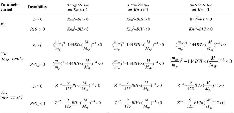
Using Equations (86) and (87) for instability conditions (S0 > 0 and ReS± > 0), Table 1 can be obtained for main sequence stars of difference masses. In this table:
As 15
7 0 10
~ × −
T
A με , B~3ρC×10−7 and
22 7
0 10 3
~ C× −
T
D με ρ , among all the terms of U and W,
only three terms AB, D and B3/2 are considerable and the rest can be ignored:
3 1 2 1 3 27 2
6 ⎟
⎟ ⎠ ⎞ ⎜
⎜ ⎝ ⎛
⎟⎟ ⎠ ⎞ ⎜⎜ ⎝ ⎛ + − = AB D B
U (83) T
T T T
T T
BV BIII BI
ε ε
ε ε
ε ε
4 32
25 4
5 . 9
5 . 2 5
13
− + =
− + =
− + =
T T T T
T T
BVI BIV BII
ε ε ε ε
ε ε
8 43
8 17
2 5 . 11
5 . 3 2
2 7
11 2
− + =
− + =
− + =
Results and Discussion 3
1 2 1 3 27 2
6 ⎟
⎟ ⎠ ⎞ ⎜
⎜ ⎝ ⎛
⎟⎟ ⎠ ⎞ ⎜⎜ ⎝ ⎛ − −
= AB D B
W (84)
Table 1. Instability conditions for various values of Knudsen number, cosmion mass and cross section
Parameter
varied Instability
τ ~τff << τrel ⇔ Kn >> 1
τ ~τff >> τrel ⇔ Kn << 1
τff <<τ < τrel ⇔ Kn ~ 1
S0 > 0 Kn0
2
–BI > 0 Kn0
2
–BIII > 0 Kn0 2
–BV > 0
Kn
ReS± > 0 Kn02–BII <0 Kn02–BIV < 0 Kn02–BVI < 0
S0 > 0 ( ) 144 ( ) 0
4 . 3− × − >
Θ
M M BI m
m p
m ( )3−144 ×( )−.4>0
Θ
M M BIII m
m p
m ( )3−144 ×( )−.4>0
Θ
M M BV m
m p m mW
(σcap=const.)
ReS± > 0 ( ) 144 ( ) 0
4 . 3− × − <
Θ
M M BII m
m p
m ( )3−144 ×( )−.4<0
Θ
M M BIV m
m p
m ( )3 −144 ×( )−.4<0
Θ M
M BVI m
m
p m
S0 > 0 ( ) 0
125
9 .4
2− × − >
Θ −
M M BI
Z ( ) 0
125
9 .4
2− × − >
Θ −
M M BIII
Z ( ) 0
125
9 .4
2− × − >
Θ −
M M BV Z
σcap (mW=const.)
ReS± > 0 ( ) 0
125
9 .4
2− × − <
Θ −
M M BII
Z ( ) 0
125
9 .4
2− × − <
Θ −
M M BIV
Z ( ) 0
125
9 .4
2− × − <
Θ −
M M BVI Z
We called the corresponding instability modes I, II,… and VI, respectively. For the sake of brevity, we summarize the results as:
1. Instability modes I, IV, V and VI occur for
population I stars in the mass range 0.24≤ ≤5
Θ M
M
for
various values of the cosmion mass and cross section. 2. The same instability modes occur for population II
stars in the mass range 0.24≤ ≤0.7
Θ M
M
. Mode II
occurs for population II stars heavier than 0.7 MΘ. 3. For heavy population I stars (M>5MΘ), instability modes I, II and V occur.
We conclude that cosmions with a mass of 4-10 Gev/c2 and scattering cross section 0.2-11×10-36 cm2, previously suggested to constitute the Galactic halo and to solve both dark matter and solar neutrino problems, may cause thermal instabilities in the core of the sun and many other main sequence stars which have captured an efficient number of cosmions.
It should be stressed that the analysis followed in this paper was a local one and only linear perturbations were taken into account. A more exact investigation must consider both a global analysis and nonlinear dynamical effects.
Such a wide range of instability modes, if present weaken the cosmion hypothesis in the mass and cross section region which is interesting in the context of the dark matter and solar neutrino problems.
References
1. Aller, L. H. and McLaughlin, D. B. Stellar Structure,
University of Chicago Press, (1965).
2. Bahcall, J. N., Basu, S. and Kumar, P. Astrophys. J., 485, L91, (1997).
3. Baker, N. Stellar Evolution. (ed.) R. F. Stein and A. G. W. Cameron, Plenum Press, New York, (1966).
4. Bouquet, A. and Salati, P. Astron. Ap., 217, 270, (1989). 5. Bouquet, A. and Salati, P. Astrophys. J., 346, 284, (1989). 6. Clayton, D. D. Principles of Stellar Evolution and
Nucleosynthesis, McGraw-Hill Book Company, (1968). 7. Cox, J. P. and Giuli, R. T. Principles of Stellar Structures,
Cordon and Breach, New York, (1968).
8. Davis, R. Jr. Encyclopedia of Astronomy and
Astruophsics, (ed.) R. A. Meyers, Academic Press, Inc., (1989).
9. Gilliland, J., Faulkner, J., Press, W. H. and Spergel, D. N.
Astrophys. J., 306, 703, (1986).
10. Faulkner, J. and Gilliland, R. L. Ibid., 299, 994, (1985). 11. Gould, A. Ibid., 321, 560, (1987).
12. Gould, A. and Raffelt, G. Ibid., 352, 654, (1990a). 13. Gould, A. and Raffelt, G. Ibid., 352, 669, (1990b). 14. Krauss, L., Freese, K., Spergel, D. N. and Press, W. H.
Ibid., 229, 1001, (1985).
15. Novotny, E. Introduction to Stellar Atmospheres and Interiors, Oxford University Press, (1973).
16. Press, W. H. and Spergel, D. N. Astrophys. J., 295, 679, (1985).
17. Raby, S. Ibid., 347, 551, (1989).
18. Raby, S. and West, G. B. Nucl. Phys., 239, 793, (1987). 19. Reeves, H. In: Aller and McLaughlin, (1965).
20. Riazi, N. Mon. Not. R. Astr. Soc., 248, 555, (1990). 21. Spergel, D. N. and Press, W. H. Astrophys. J., 294, 663,