Stability and Performance Attainment with Fixed Order Controller Using Frequency Response

(1)

Please cite this article as: M. Mohammadizadeh, B. Pourabbas, K. Foroutani, M. Fallahian,Conductive polythiophene nanoparticles deposition on transparent PET substrates: effect of modification with hybrid organic-inorganic coating, International Journal of Engineering (IJE), TRANSACTIONS A: Basics Vol. 28, No. 4, (April 2015) 553-560

International Journal of Engineering

J o u r n a l H o m e p a g e : w w w . i j e . i r

Stability and Performance Attainment with Fixed Order Controller Using Frequency

Response

H. Parastvand, M. J. Khosrowjerdi*

Department of Electrical Engineering, Sahand University of Technology, Tabriz, Iran

P A P E R I N F O

Paper history: Received 22 March 2014

Received in revised form 05 November 2014 Accepted 29 January 2015

Keywords: Fixed Order Controller Linear Matrix Inequality Frequency Domain Inequality Performance Attainement

A B S T R A C T

Recently, a new data driven controller synthesis is presented for calculating the family of stabilizing first, second and fixed order controllers using frequency respons. However, this method is applicable just for plants that can guarantee some smoothness at the boundary of the resulted high dimension LMI. This paper solve that issue and extends the approach to fixed order controllers guaranteeing some performance criteria which are applicable for the more general types of plants. It is shown that knowing the frequency response of plant is sufficient to calculate the stabilizing fixed order controllers from a set of convex linear inequalities. TheH¥norm on sensitivity and complementary sensitivity functions are satisfied from some frequency domain inequalities (FDI) that could be examined from frequency response data. The usefulness of the proposed approach is illustrated by an academic example.

doi: 10.5829/idosi.ije.2015.28.04a.09

1. INTRODUCTION1

Fixed order controller is the subject of many studies in literature. Toward other analytical methods such as theorem, calculating the low order controller is the main advantage of fixed order controller design approaches. The most of these procedures lead to first or second order controllers [1-4] that are more conventional controllers toward other high order controllers. In fact, 90 percent of industrial controllers are currently belong to the family of PID controllers (for example see [5]). The PID

A polynomial method is implemented to calculate a fixed order controller so that the closed loop poles reside within a given region of complex plane [1]. A parameter space approach is presented [2] by constrained variance and minimum variance PID controller design for LTI models. The technique is based on plant mathematical model and noises. Using a version of Hermite-Biehler Theorem extended to

1_{*Corresponding Author}_’_{s Email:}_{[email protected]}_(M.J.

Khosrowjerdi)

quasipolynomials for first order plants, the complete family of stabilizing PID controllers is determined in [3]. Also, a modified chaotic genetic algorithm has been used to optimize the coefficients of PID controller [4]. Some optimization based approaches to PI/PID controller design are reviewed in literatures [6, 7]. These approaches are faced to the problem of non-convexity of the design parameters. A global lower bound on the achievable PID performance, defined in terms of output variance, is presented [8] that leads to solving a series of convex programs using sum of square programming. Another convex optimization of fixed order stabilizing controllers for systems with polytopic uncertainty is presented [9] as a linear matrix inequality using Kalman-Yakubovich-Popov (KYP) Lemma. Based on decoupling at singular frequencies, the algorithm of calculating the family of stabilizing PIDs is presented [10] in which nonconvex stability regions are built up by convex polygonal slices. All of these approaches are model based and need to mathematical model or time domain data of plant.

(2)

iterative feedback tuning [14] and extremum seeking [15] are already presented in the literature. A good review of these approaches could be found in literature [15]. Adaptive control is another model free approach [16, 17] that similar to other mentioned model free techniques relies on time domain data of plant. The first frequency based controller synthesis was based on loop shaping of open loop transfer function using Nyquist, Bode and Nicholz diagrams. The most practical issue in the frequency domain approaches is the difficulty in measuring the frequency response of unknown plants which are composed of hard nonlinear dynamics that triger high order harmonics. Also, the measurements are usually faced to measring noises.

Recently a new model free controller synthesis based on frequency response of plant is proposed [18] that can achieve to the set of stabilizing fisrt and second order controllers that satisfies some performance considerations. That approach is extended to simultaneously stabilizing [19], robust PID synthesis for plants with single uncertainty [20], robust stability for unstructured uncertainties [21] and fixed order controllers that can satisfy a particular performance criteria [22]. However, this criteria has a general drawback. In fact, since the approach applies a sort of gridding on a parameter of the performance criteria, the scope of solution is limited to plants that can guarantee some smoothness at the boundary of the resulted high dimension LMI. All the reviewed approaches have one or some of these limitations: (1) The mathematical model of plant is needed; (2) Some plants could not be stabilized by first or second order controllers [23]; (3) Some optimization approach may lead to a non-convex problem; (4) Some approach is applicable for plants that can that can guarantee some smoothness at the boundary of the resulted LMI. In the proposed approach of this paper, it is illustrated that for stability achievement, it is sufficient to examine the feasibility of some linear inequalities in terms of controller parameters. Many performance specifications can be achieved by satisfying H¥norm of sensitivity and complementary

sensitivity functions. But there is a problem in dealing with LMI in a model free manner. It isn’t possible to synthesis controller with these performance considerations using frequency response data. The frequency domain inequalities are model based and there isn’t any FDI that can be solved using spectral model of plant. The contribution of the paper is proposing a new approach to satisfy the performance specifications using FDIs. In fact the performance considerations are transformed to some linear inequalities in terms of controller parameters and frequency. The feasibility of this problem can be analyzed using new FDIs by MATLAB. Moreover, since the proposed approach does not rely on gridding, it is applicable to more general types of plants.

This paper is organized as follows. In section 2, the idea of fixed order controller design presented in [22] is reviewed. Section 3 illustrates how to achieve the performance specifications using frequency response data. In section 4, the effectiveness of the proposed approach is illustrated by an academic example. Some concluding remarks are mentioned in section 5.

2. FIXED ORDER CONTROLLER SYNTHESIS

In this section, we propose an algorithm to calculate the stabilizing fixed order controllers in the structure of Figure 1. The control objective is to synthesis a lowest order stabilizing controller that satisfiesH¥norm of

sensitivity and complementary sensitivity functions. First, some mathematical preliminaries will be presented. Consider a real rational function

( ) ( )

( )

A s P s

B s

= ₍₁₎

where, A s( ) and B s( )_{are polynomials with real} coefficients and degrees m and n, respectively. We assume that A s( )and B s( )have no zero on jw axis. Let

z+_and

p+ _{( ,}_{z p}- -₎_{determine the number of open right}

half plane (RHP) (open left half plane (LHP)) zeros and poles of P s( ). Also let DÐP j

( )

w denotes the net change in phase as ω runs from 0 to +¥. Then, we have

( )

(( ) ( ))

2

P jw p z- z+ p- p+

DÐ = - - - (2)

The (Hurwitz) signature of P s( )is defined as

( )

P z z

(

p p

)

2 P j

( )

s w

p

- + - +

= - - - = DÐ (3)

sinceP s( )has no pole and zero on jwaxis, we have

( )

P (n m) 2(z p )

s = - - - +- + (4)

or

( )

P r_p 2(z p )

s _{= - -} +_- + ₍₅₎

where, r_pis the relative degree of plant P s( )and can be obtained from high frequency slope of bode magnitude. The only available data is the frequency response of unknown plantP s( )for w³0. The frequency response of plants is as

( )

j ( )

( )

r i

c=P jw ef w =P w +jP w (6)

where, P_r( )w and P_i( )w denote the real and imaginary parts of Pi( )w , respectively. Assume that the real,

(3)

0 1 1

0=w <w <¼<wl- <wl= ¥. (7)

Lemma 2.1: for n m- is even

0 ( 1)

( ) ( ( ( ))2 ( 1) ( ( )) ( 1) ( ( )))( 1) ( ( ))

j

r r j

l l

r l i

P sgn P sgn P

sgn P sgn P

s w w

w

-= S

-+ - - ¥ (8)

and for n m- odd

0

( 1)

( ) ( ( ( ))

2 ( 1) ( ( )))( 1) ( ( )).

r

j l

r j i

P sgn P

sgn P sgn P

s w

w

-=

+ S - - ¥ (9)

Let the controller in the structure of Figure 1 be as

( )

(

)(

)

(

)(

)

1 _{2( 1)}

2 0

1 2 ( 3)

1 2 1

3 2( 1) 2

0

1 2 ( 3)

1 2 1

:

1 1 (1 )

:

1 1 (1 )

N i i i N N i i i N s s N even

s sT sT sT

C s

s s

N odd

s sT sT sT

r r r

- ₊ = + -+ = + -ì

+ + å

ï

ï ₊ ₊ _{¼ +}

ï = í

ï ₊ _{+ å}

ï

ï + + ¼ +

î

(10)

where, r r1, , , 2¼ ri+3, T T1 2, , , ¼TN-1and Nare design parameters, arbitrary constants and the order of controller, respectively. Now consider N be even. Let

( ) (

)(

)

( )

1 2 1 1

( 1)

2 _{2( 1)}

2 ( 3)

0 1

.

1 (1 N )

N

i i i

F s s sT s T

P T s s s s r r r -+ + =

= + + ¼ +

+ + å (11)

Lemma 2.2: The closed loop stability is equivalent to the below equality

( )

(

F s

)

n m 2z N.

s _{= - +} +₊

(12)

Let F s

( )

=F s P s( ) ( )- and write

( )

r

(

, ,1 3, 4, , i 3

)

i

(

, 2

)

.

F w =F w r r r ¼ r+ + j Fw w r (13)

Consider Fi

(

w r, 2

)

=0and define

( )

2 2 ( : ) i r

aP j bP j

g P j w w r w w w -= = ₍₁₄₎

in which, a and b can be obtained from the denominator of controller as

(

1 1

) (

1 N

)

jw + j Tw ¼ + j Tw = +a jb ₍₁₅₎

Unknown Plant P(jω) Fixed Order

Controller

+ _{_}

r u y

Figure 1. The feedback structure of plants with fixed order

controller.

And define J =sgn F[ i(¥-,r2)]wherer2min<r2*<r2max.

Theorem 2.1: Let w1<w2< ¼ <wl-1denote the distinct frequencies of odd multiplicities which are solutions to

(

, 2

)

0

i

F w r = . Determine string of integers

0 1 2, , , ,l

I=é_ëi i i ¼iù_û where i_tÎ -

{ }

1,1 such that for n m

-even:

( 1) ( 1)

0 1 ( 1)

[ ... ( 1)l 2 ( 1) ]( 1)l l 2

l l

i - + + -i - i _- - i - - J n m= - + z++N (16)

and for n m- odd:

( ) 1 ( ) 1

0 1 1 2 1 1 2

l l

l

i i - i -J n m z+ N

-é _{- +¼+ -} ù _- _{= -} ₊ ₊

ê ú

ë û (17)

and il=sgn F( r

(

¥-, ,r r r₁ ₃, ₄, ,¼ri+₃

)

). Then forr2=r*2, the ( ,r r r1 3, 4, ,¼ ri+3) values corresponding to closed loop stability can be found by solving the problem of feasibility of 1 1 0 0 0 0 0 0 0 0 0 0 0 0 0 r r rt f f f æ ö ç ÷ ç ÷ ç ÷ ç ÷ ç ÷ ç ÷ è ø p O M O M M (18)

where, f_r₁<0 , 1,2, ,i= ¼t are corresponding to inequalities

(

, , ,1 3 4, , 3

)

0

r t i t

F w r r r ¼r+ i > (19)

and it’s are taken from strings satisfy Equations (16) or (17) and wt’s are taken from the Equation (14). The proof for Lemmas 2.1 and 2.2 and Theorem 2.1 can be found in [18]. This theorem can be proved using the stability criteria of Equation (18) and applying Lemma 2.1 to compute the signature of F s( ).

Theorem 2.2: The necessary condition for PID

stabilizing is that there exists r2 such that Equation (14) has at least R distinct roots of odd multiplicities such that

2

1 : 2

2 1

1 : . 2

n m z N

R if n m even

n m z N

R if n m odd

+

ì _³ - + + _-

-ïï í

- + + +

ï ³ -

-ïî

(20)

(4)

( ) ₍ H j₎₍₁( )₍ ₎₎

P j

C j C j

w w

=

- (21)

The next theorem illustrates how to calculate the number of right half plan (RHP) zeros and poles of plant

( )

P s . As it will be shown, there is no need to plant mathematical model to calculate RHP poles and zeros.

Theorem 2.3: The number of RHP zeros and poles can

be obtained from

1

[ 2 ( )]

2 p C C

z+₌ _{- -}r r _- z+_-s H ₍₂₂₎

( )

1

2

2 C C

p+₌ _és P _-s H _-r _ù_- z+

ë û (23)

where, zC+ and rC are the number of RHP zeros and the relative degree of C s( ), respectively.

The proof for Theorems 2.2 and 2.3 can be found in research [22]. The procedure of calculating the lowest order controllers with frequency response data is summarized in the following algorithm.

Algorithm 2.1: Calculating the lowest order controllers

with frequency response.

1- Determine the relative degrees of plant from high frequency slope of Bode magnitude diagram. 2- Determine z+ for every plant from (4). 3- Set N=1.

4- Determine the range of r2 from Theorem 2.2. 5- If there is not any r2that satisfies the conditions

of Theorem 2.2 then set N N= +1and go to Step 4, else go to the next step.

6- For *

2 2

r =r solve (14) and obtain roots with odd multiplicity as w1<w2< ¼ <wl-1.

7- Let w1=0and wl = ¥ and define

(

2

)

[ i , ]

J ₌sgn F _¥- r _{. Determine}

0 1, , ,l 1 i i ¼i- from Equations (16) or (17).

8- Forr2=r*2, determine the ( ,r r r1 3, 4, ,¼ ri+3) values from Equation (18).

9- Change the value of r2 and go to Step 4 to obtain another stabilizing PID controller.

3. PERFORMANCE CONSIDERATION WITH FIXED ORDER CONTROLLER

Many performance attainment problems for plant P s( ) can be cast as the problem of achieving an H¥norm

specification on the sensitivity and complementary sensitivity functions [18]. In Section 2, the stabilizing controllers obtained from solving the feasibility problem

of the linear matrix inequality [18]. Here, the main contribution of the paper is presented. To obtain the lowest order controllers that achieves to stability and performance, another constraints are needed to add to Equation (18), but there isn’t any linear performance condition that can be examined by frequency response data. In the other hand, every FDI needs to state space or transfer function of the plant. In the next theorem and the following corollaries, we transform the problem of performance attainment to the feasibility problem of some linear inequalities that can be examined by new FDIs.

Theorem 3.1: Consider the structure of Figure 1 with controller of Equation (10). Then:

(1) The closed loop system achieves to the H¥norm of

sensitivity function, i.e. 1

1+c s P s( ) ( ) <g , if the

controller parameters satisfy one of the below sets of inequalities for w³0:

( ) ( )

1

1 1 : 0

1 1 0

Re CP Im CP h Re CP Im CP

Re CP Im CP

g

- + + + - = <

+ + >

+ - + >

ì ï ï í ï ïî

(24)

( ) ( )

2

1

1 1 : 0

1 1 0

Re CP Im CP h Re CP Im CP

Re CP Im CP

g

- + + + - = <

+ + >

+ - + <

ì ï ï í ï ïî

(25)

(

)

(

)

(

) (

)

(

)

(

)

3

1

1 1 : 0

1 1 0

Re CP Im CP h

Re CP Im CP

Re CP Im CP

g

- + + + - = <

+ + <

+ - + >

ì ï ï í ï ïî

(26)

(

)

(

)

(

) (

)

(

)

(

)

4

1

1 1 : 0

1 1 0

Re CP Im CP h

Re CP Im CP

Re CP Im CP

g

- + + + - = <

+ + <

+ - + <

ì ï ï í ï ïî

(27)

(2) The closed loop system achieves to the H¥norm of

complementary sensitivity function, i.e.

( )

( ) '

1 ( ) ( )

C s P s

C s P s <g

+ , if the controller parameters satisfy

one of the below sets of inequalities for w³0:

( ) ( )

' : 1 0

0 0 Re CP Im CP J Re CP Im CP

Re CP Im CP

g g

- + - = <

<

+ >

ì ï ï í ï ï î

(28)

( )

( ) ( )

( )

' : 2 0

0 0

Re CP Im CP J Re CP Im CP

Re CP Im CP

g g

- + = <

>

+ <

(5)

( )

( ) ( )

( )

' : 3 0

0 0

Re CP Im CP

g g

- - - = <

<

- >

(30)

( )

( ) ( )

( )

': 4 0

0 0

Re CP Im CP

g g

+ + = <

<

+ <

(31)

Proof: for part (1) we have the performance constraint as

( )

(

)

2 2

1

1 ( )

1

1 (1 ) :

C s P s

Re CP Im CP d

g

+ >

=> + + + > =

(32)

Leta=Re(1+C j

( )

w P j( w)) and b Im= (1+C j

( )

w P j( w)). Then from _a2₊_b2_>_d2_{we have two following cases:} 1) If ab>0, then _a2₊_b2_>₍_{a b}_- ₎2_{and we have:}

· If (a b- >) 0, then the performance condition

transforms to the constraint (a b- >) d that is equivalent to Equation (24).

· If (a b- <) 0, then the performance condition

transforms to the constraint

(

a b-

)

< -d that is equivalent to Equation (25).

2) If ab<0, then _a2₊_b2_>₍_{a b}₊ ₎2_{and we have:}

· If (a b+ >) 0, then the performance condition

transforms to the constraint (a b+ >) d that is equivalent to Equation (26).

· If (a b+ <) 0, then the performance condition

transforms to the constraint

(

a b+

)

< -d that is equivalent to Equation (27).

For part (2) of theorem, we have the performance constraint as

( )

( ) '

1 ( ) .

C s P s

C s P s <g

+ (33)

From part (1) of theorem we have

( )

1

( )

1 ( ) 1 ( )

C s P s

C s P s < =>g C s P s <g

+ + (34)

It can be written

'

2 2 2 2 2

e f g h e f h

g

+ < = => + < (35)

1) If ef >0, then ₍_e2₊ _f2_{) (}_> _e₊ _f₎2_{and we have:}

· If (e f+ ) 0> , then the performance condition transforms to the constraint (e f+ )<h that is equivalent to Equation (28).

· If (e f+ ) 0< , then the performance condition transforms to the constraint

(

e+ f

)

> -h that is equivalent to Equation (29).

2) If ef <0, then ₍_e2₊ _f2_{) (}_> _e_- _f₎2_{and we have:}

· If (e f- ) 0> , then the performance condition transforms to the constraint (e f- )<h that is equivalent to Equation (30).

·

If (e f- ) 0< , then the performance condition transforms to the constraint

(

e- f

)

> -h that is equivalent to Equation (31).

The following two corollaries introduce two FDIs to obtain lowest order controllers that satisfy H¥norm on

sensitivity and complementary sensitivity functions.

Corollary 3.1: To satisfy stability and H¥norm on

sensitivity function, the feasibility of the following FDI must be satisfied:

1

2

0 0 0 0 0 0 0 0

0 0

0 0 ₀

0 0 0 0

0

0 0 0

r r

rt i

f f

f h

æ ö

ç ÷

è ø

O _p

M M

O

M M (36)

where, h_i , 1, , 4i= ¼ are corresponding to Equations (24-27). For every ℎ and every frequency a set of controller parameters will be obtained. Obviously, we select the controller that leads to best closed loop response.

Corollary 3.2: To satisfy stability and H¥norm on

sensitivity and complementary sensitivity functions, the feasibility of the following FDIs must be satisfied:

1

2

0 ₀ ₀ ₀ ₀

0 0 0 0 0

0

0 0 0 0 0

0 0 0 ₀ 0

r r

rt i

i

f f

f h

J

æ ö

ç ÷

è ø

O

M M O M M M p (37)

where, Ji , 1, , 4i= ¼ are corresponding to Equations

(28)-(31). For every hi, Ji and every frequency w, a set of controller parameter will be obtained. Obviously, we select the controller that leads to best closed loop response.

4. SIMULATION

(6)

( )

1 2 3 2 (1 )

s s

C s

s sT

r +r +r

=

+ (38)

where, T=1. From Equation (20) we have

2 2 1 1. 2

R³ + - = (39)

For r2=10, from Figure 3 w1=26.96 and the corresponding inequalities for stability region are

1

1 3

0

723 497 0

r

r r

> ì

í _- _- _<

î (40)

Choosing r1=150 and r3=10 is led to step response of Figure 4-a. Obviously, these parameters are corresponding to only stabilizing region and there isn’t any performance consideration. As you see in Figure 4, the overshoot is 50% and the rise and settling times are large. For the problem of satisfying H¥norm of

sensitivity function, the feasibility of Equation (36) must be examined through checking Equations (24)-(27) for w>0. This, in turn, will lead to a high dimension LMI in MATLAB. The simulation is accomplished and the parameters are obtained as r₁=33.9978 and r₃= -1

So the corresponding controller is

( )

33.9978 10 2

(1 )

s s C s

s s

+

-=

+ (41)

And the corresponding step response is shown in Figure 4-b. There isn’t overshoot in this case but still the rise and settling times are large. For the problem of satisfying H¥norm of sensitivity and complenetray

sensitivity function, the feasibility of Equation (37) must be examined through checking Equations (28-31) for w>0. This, in turn, will lead to a high dimension LMI in MATLAB. The simulation is accomplished and the parameters are obtained as r1=9.0228 and

3 0.1

r = - and the corresponding controller is

( )

9.0228 10 0.12. (1 )

s s

C s

s s

+

-=

+ (42)

Figure 1. The Bode diagram of plant P s

( )

.

Figure 2. The plot of function g( )w

Figure 3. Step responses corresponding to (a), stabilizing

controller without any performance consideration; (b), stabilizing controller of Equation (41) which satisfies H¥

norm of sensitivity function; (c), stabilizing controller of Equation (42) which satisfies norm of sensitivity and complementary sensitivity functions.

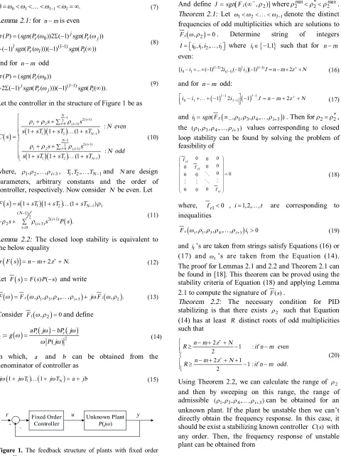
Figure 5. The magnitude of sensitivity and complementary

sensitivity functions corresponding to Equation (42).

The corresponding step response is shown in Figure 4-c. The rise and settling time are improved and there isn’t overshoot in the response. Finally, the magnitude plot of sensitivity and complementary sensitivity functions, i.e. | ( ) |S s and | ( ) |T s , with controller as the form of Equation (42) are shown in Figure 5. It could be concluded that the proper shaping of these diagrams is resulted to better specifications in the step response of the plant with frequency response of Figure 2.

-80 -60 -40 -20 0 20

M

a

gn

itu

d

e (

d

B)

100 101 102 103 104

-180 -135 -90 -45 0

P

hase

(

d

eg)

Bode Diagram

Frequency (rad/s ec )

0 5 10 15 20 25 30 35 40

-5 0 5 10 15 20 25

Frequency (w)

g(

w

)

w=26.96 g(w)=10

0 5 10 15 20 25 30 35 40 45 50

0 0.5 1 1.5

y

(a)

0 5 10 15 20 25 30 35 40 45 50

0 0.5 1 1.5

y

(b)

0 5 10 15 20 25 30 35 40 45 50

0 0.5 1 1.5

Time (s)

y

(c)

10-2 100 102

-120 -100 -80 -60 -40 -20 0 20

M

ag

nit

ude

(

d

B)

Bode Diagram

Frequency (rad/sec)

(7)

Other admissible parameters can be obtained by sweeping on the admissble range of r2. All resulted controllers can guarantee the performance criteria used in this paper. However, solving Equations (36) and (37) may result in a non-minimum phase controller.

For the time being, there has not been found any general rule on the effect of sweeping on controller parameters. Since the controller parameters must be selected among a set of convex inequalities through Equations (24) to (31), the computed parameters by MATLAB might construct a conservative controller. This is a work in progress to find the optimal parameters among the admissible range. There has been provided lots of examples on this issue in literature [24].

5. CONCLUDING REMARKS

Through the paper, an algorithm for calculating the fixed order controller proposed using only frequency domain data is reviewed. The previous technique was applicable just for plants that can guarantee some smoothness moothness at the boundary of the resulted high dimension LMI. This paper solve that issue and extends the approach to fixed order controllers guaranteeing some performance criteria which are applicable for the more general types of plants. It is shown that the performance specifications such as H¥

norm of sensitivity and complementary sensitivity functions can be examined by new linear inequalities in terms of controller parameters and frequency. This is the important feature of these constraints by which the problem of stabilizing controller synthesis with performance consideration can be transformed to the feasibility problem of new FDIs that could be analyzed using frequency response data.

Another important feature of the proposed approach is that there is no need to exact data on the whole range of frequency response. In fact, exact data are needed just at low frequency band and beyond which data might be rough or approximated.

Althought there are some useful techniques for measuring the frequency response such as attaining the input-output data using Fourier analysis, virtual sine sweeping, spectrum analyzer, network analyzer or using audio sine-wave generators and the sine function of function generators, but measuring the frequency response of plants with hard nonlinearity is still a challenging issue. This needs to more improvement to the measuring technologies and instruments.

6. REFERENCES

1. Yang, F., Gani, M. and Henrion, D., “Fixed-order robust controller design with regional pole assignment”, IEEE

Transaction, Vol. 52, (2007), 1959-1963.

2. Dickinson, P. B., Shenton, A. T., “A parameter space approach to constrained variance PID controller design”, Automatica., Vol. 45, (2009), 830-835.

3. Silva, G. J., Datta, A. and Bhattacharyya, S. P., “New Results on the Synthesis of PID Controllers”, IEEE Transaction, Vol. 47, (2002), 241-252.

4. Mahmoudzade, A., Mojallali, H., and Pourjafari., “An optimized PID for capsubots using modified chaotic genetic algorithm”,

International Journal of Engineering., Vol. 27, (2014), 1377-1384.

5. Samuel Rajesh babu, R., Deepa, S., and Jothhivel, S., “A closed loop control of quadratic boost converter using PID controller”,

International Journal of Engineering, Vol. 27, (2014), 1653-1662.

6. Pedret, C., Vilanova, C., Moreno, R. and Serra, I., “A refinement procedure for PID controller tuning”, Com-puters and Chemical

Engineering, Vol. 26, (2002), 903-908.

7. Toscano, R., “A simple robust PI/PID controller design via numerical optimization approach”, Journal of Process Control, Vol. 15, (2005), 81-88.

8. Sendjaja, A. Y. and Kariwala, V., “Achievable PID performance using sums of squares programming, Journal of Process

Control”, Vol. 19, (2009), 1061-1065.

9. Khatibi, H., Karimi, A. and Longchamp, R., “Fixed-order controller design for polytopic systems using LMIs”, IEEE

Transaction., Vol. 53, (2008), 428-434.

10. Bajcinca, N., “Design of robust PID controllers using decoupling at singular frequencies”, Automatica., Vol. 42, (2006), 1943-1949.

11. Astrom, K. J. and T. Hagglund, Automatic tuning of simple regulators with specifications on phase and amplitude margins,

Automatica., Vol. 20, (1984), 645-651.

12. Voda, A. A. and Landau, I. D., “A method for the auto-calibration of PID controllers”, Automatica, Vol. 31, (1995), 4153.

13. Saeki, M., Takahashi, A., Hamada, O. and Wada, N.,

“Unfalsified parameter space design of PID controllers for nonlinear plants” ,in Proc. IEEE Int., Symp. CACSD, Taipei, Taiwan, 1521-1526, (2004).

14. Hjalmarsson, H., Gevers, M., Gunnarsson, S. and Lequin, O.,

“Iterative feedback tuning: Theory and applications”, IEEE

Control System Magazine., Vol. 18, (1998), pp 2641.

15. Killingsworth, N. J. and Krstic, M., “PID tuning using extremum seeking”, IEEE Control System Magazine., (2006), 70-79.

16. Coelho, L.D.S. and Coelho, A.A.R., “Model-free adaptive control optimization using a chaotic particle swarm approach”,

Chaos, Solitons and Fractals, Vol. 41, (2009), 2001-2009.

17. Baleghi Damavandi, Y., Mohammadi, K., Upegi, A., and Thoma, Y., “On feasibility of adaptive hardware evolution for emergent fault tolerant communication”, International Journal

of Engineering, Vol. 27, (2014), 101-112.

18. Keel, L.H. and Bhattacharyya, S. P., “Controller synthesis free of analytical model: Three term controllers”, IEEE trans.

Automat. Control, Vol. 53, (2008), 1353-1369.

19. Parastvand, H., Khosrowjerdi, M.J, Akbari Alvanegh, A., “A new model free approach to simultaneously stabilizing”, 19th Iranian Conference on Electrical Engineering , Tehran, Iran (2011), 84-93.

20. Parastvand, H. and Khosrowjerdi, M.J, “A new model free approach to robust PID controller synthesis”, Journal of Control

Engineering and Applied Mathematics, Vol. 16, (2014), 84-93.

(8)

Frequency Domain Information”, International Journal of

Systems Science, Manuscript submitted for ppublication (2015).

22. Parastvand, H. and Khosrowjerdi, M.J, “Controller synthesis free of analytical model: fixed order controllers”, International

Journal of Systems Science, Vol. 46, (2015), 1208-1221.

23. Lee, S.C., Wang, Q.G. and Xiang, C., “Stabilization of all-pole unstable delay processes by simple controllers”, Journal of

Process Control, Vol. 20, (2010), 235-239.

24. Parastvand, H. and Khosrowjerdi, M.J, “Controller synthesis free of analytical model: frequency domain approach”, MS Thesis, Sahand University of Technology, (2010).