A NEW APPROACH TO APPROXIMATE COMPLETION
TIME DISTRIBUTION FUNCTION OF STOCHASTIC
PERT NETWORKS
S. M. T. Fatemi Ghomi
Department of Industrial Engineering, Amirkabir University of Technology Tehran, Iran, [email protected]
M. Rabbani
Department of Industrial Engineering, Faculty of Engineering, Tehran University Tehran, Iran, [email protected]
(Received: December 9, 1998 – Accepted in Final Form: October 5, 2001)
Abstract The classical PERT approach uses the path with the largest expected duration as the critical path to estimate the probability of completing a network by a given deadline. However, in general, such a path is not the most critical path (MCP) and does not have the smallest estimate for the probability of completion time. The main idea of this paper is derived from the domination structure between paths that was presented by Soroush for the first time. This paper develops this domination structure and its properties, which make Soroush’s algorithm work faster in some cases. Then a labeling algorithm is presented that is able to compute the MCP from starting node of the network to any node of the network. Also, suitable and practical completion time distribution function estimation is defined. In many cases, the estimation is obtained by the developed method is better than that of Soroush’s. To clarify the point, some examples are given. Finally, conclusions are presented.
Key Words PERT, Most Critical Path, Stochastic Network, Completion Time, Distribution Function, Approximation
ﻩﺪﻴﻜﭼ
ﺍﺭﻥﺎﻣﺯﺕﺪﻣﻱﺭﺎﻈﺘﻧﺍﺵﺯﺭﺍﻦﻳﺮﺘﮔﺭﺰﺑﺎﻫﺮﻴﺴﻣﺮﻳﺎﺳﻪﺑ ﺖﺒﺴﻧﻪﻛﻱﺮﻴﺴﻣﺯﺍﻚﻴﺳﻼﻛﺕﺮﭘﺩﺮﻜﻳﻭﺭ
ﺺﺨﺸﻣﺪﻋﻮﻣﻑﺮﻇﺭﺩﺍﺭﻪﻜﺒﺷﻞﻴﻤﻜﺗﻝﺎﻤﺘﺣﺍﺎﺗﺩﺮﻴﮔﻲﻣﻩﺮﻬﺑﺩﺭﺍﺩ
ﺪﻧﺰﺑﻦﻴﻤﺨﺗ .
،ﻲﻠﻛﺖﻟﺎﺣﺭﺩ،ﻝﺎﺣﺮﻫﻪﺑ
ﻳﺮﺗ ﻞﻤﺘﺤﻣ ﻱﺮﻴﺴﻣ ﻦﻴﻨﭼ ﻦ
ﻲﻧﺍﺮﺤﺑ ﺮﻴﺴﻣ )
MCP (
ﻱﺍﺮﺑ ﻦﻴﻤﺨﺗﻦﻳﺮﺘﻜﭼﻮﻛ ﺯﺍ ﻭﺖﺴﻴﻧ ﻞﻴﻤﻜﺗ ﻥﺎﻣﺯ ﻝﺎﻤﺘﺣﺍ
ﺖﺴﻴﻧﺭﺍﺩﺭﻮﺧﺮﺑ .
ﺎﻫﺮﻴﺴﻣ ﻦﻴﺑﺎﻣﺐﻟﺎﻏﺭﺎﺘﺧﺎﺳﺯﺍﻪﻟﺎﻘﻣﻦﻳﺍ ﻩﺪﻤﻋﺮﻈﻧﻪﻄﻘﻧ ﻪﻛ
ﺍﺭﻥﺁﺵﻭﺮﺳ ﺭﺎﺑﻦﻴﺘﺴﺨﻧﻱﺍﺮﺑ
ﺩﺮﻴﮔﻲﻣﺖﺌﺸﻧﺖﺳﺍ ﻩﺩﺮﻛﺡﺮﻄﻣ .
ﻪﻌﺳﻮﺗﺍﺭﻥﺁﺹﺍﻮﺧﻭﺐﻟﺎﻏﺭﺎﺘﺧﺎﺳﻦﻳﺍﻪﻟﺎﻘﻣﻦﻳﺍ ﻲﻣﺐﺟﻮﻣﻪﻛﺪﻫﺩﻲﻣ
ﻢﺘﻳﺭﻮﮕﻟﺍﻱﺩﺭﺍﻮﻣﺭﺩﺩﻮﺷ
ﺪﻨﻛﺭﺎﻛﺮﺘﻌﻳﺮﺳﺵﻭﺮﺳ .
ﻳﺲﭙﺳ
ﺩﻮﺷﻲﻣﻪﺋﺍﺭﺍﻲﻧﺯﺐﺴﭼﺮﺑﻢﺘﻳﺭﻮﮕﻟﺍﻚ ﻪﺒﺳﺎﺤﻣﻪﻛ
MCP
ﺩﺯﺎﺳﻲﻣﺮﻳﺬﭘﻥﺎﻜﻣﺍﻪﻜﺒﺷﺭﺩﻱﺍﻩﺮﮔﺮﻫﺎﺗﻪﻜﺒﺷﻉﻭﺮﺷﻩﺮﮔﺯﺍﺍﺭ .
ﻥﺎﻣﺯﻊﻳﺯﻮﺗﻊﺑﺎﺗﺯﺍﻲﻨﻴﻤﺨﺗ،ﻦﻴﻨﭽﻤﻫ
ﺩﻮﺷ ﻲﻣ ﻒﻳﺮﻌﺗﺐﺳﺎﻨﻣ ﻭ ﻲﻠﻤﻋ ﻞﻴﻤﻜﺗ .
ﻦﻴﻤﺨﺗ ﺯﺍ ﺮﺘﻬﺑ ﻪﺘﻓﺎﻳﻪﻌﺳﻮﺗ ﺵﻭﺭ ﺯﺍ ﻪﻠﺻﺎﺣ ﻦﻴﻤﺨﺗ ،ﻱﺩﺭﺍﻮﻣ ﺭﺩ
ﺖﺳﺍﺵﻭﺮﺳ .
ﺿﻮﻣﻪﻜﻨﻳﺍﻱﺍﺮﺑ ﺖﺳﺍﻩﺪﺷﻥﺍﻮﻨﻋﻲﻳﺎﻬﻟﺎﺜﻣ،ﺩﻮﺷﺢﺿﺍﻭﻉﻮ
. ﺪﻧﻮﺷﻲﻣﻪﺋﺍﺭﺍﺞﻳﺎﺘﻧ،ﺎﺘﻳﺎﻬﻧ .
INTRODUCTION
A PERT network is an acyclic, connected and directed graph. The network has one starting and one terminal node. PERT networks are useful
models for project planning and control. Duration of all activities is positive random variables with known probability distribution. The completion
series-parallel networks of mini-networks. They allow the mini-networks to be a single arcs or Wheatsone bridge type of networks. They develop formulae to replace a Wheatsone bridge type of network by a single arc with appropriate distribution function. Ringer [2] generalizes Harthley and Wortham’s work by allowing double Wheatsone bridges as mini-networks. When all activity durations are exponential, PERT networks are formulated as a continuous time Markov chain (CTMC), and the project completion time can be thought of as a particular first passage time in this CTMC. Kulkarni and Adlakha [3] have taken this approach. Martin [4] has provided a systematic way of implementing convolution and multiplication operations, where probability distribution of each activity is polynomial.
Dodin [5] derives a bound for F(t) with the assumption of independent random variables at network. Robillard and Trahan [6] derive a lower bound using Laplace transforms, assuming that activity times are independent. Also, Kleindorfer [7] provides upper and lower bounds for F(t) where discrete random variables are considered. Van Slyke [8] estimates the mean of F(t) by means of critical index of paths. Sculli [9] derives an approximation for the mean and variance of F(t) where normal probability distributions are considered.
Kamburowski [10] obtains upper and lower bounds for mean and lower bounds for variance of F(t). Fulkerson [11], Clingen [12], Elmaghraby [13], Robillard and Trahan [14], Lindsey [15], Dodin [16], derive bounds for the mean of F(t) for some cases.
About MCP identification, Martin [4] defines criticality index of a path but does not present a method for its computation. Sigal, Pritsker and Solberg [17] derive a method that stems from Monte Carlo simulation. Also, Fisher and Goldstein [18] present an algorithm to calculate it. Elmaghraby and Dodin [19] discuss criticality of activities. Dodin [20] derives a method to identify K most critical path in a network. In the next sections, because of dependency of our approach on Soroush’s algorithm [21], his work is discussed and the domination structure presented by him is developed. Then a labeling algorithm for MCP identification is derived at a given time. At the
end, a new approach on approximate F(t) based on MCP is derived. Finally, numerical analysis is made and conclusion is presented.
PROBLEM IDENTIFICATION
Let G (V,A) be a PERT network where V is the set of nodes and A is the set of arcs and
V =n A, =m Let. R=
{
r1,....,rR}
is the set of paths between v1 and vn. The network is stochasticin the sense that all activity times tk , ak ∈A are
random variables. The duration T* of the PERT
network is;
{ }
,r Rj r k
a k
t T
where , T max
T j j j
R r *
j ∑ ∈
∈ =
= ∈ (1)
Then, the probability to complete the project by a given deadline t, is;
{ }
T t p max{ }
T t p{
T t, r R}
p j j j
R j r
* = ≤ ∀ ∈
≤ =
≤
∈ (2)
To determine an upper bound onP T
{
*≤t}
, let us rewrite (2) as:{ }
T t p{
T t}
p{
T t r r R T t}
r Rp *≤ = i ≤ . j ≤ ,∀ j≠ i∈ | i≤ , i∈
(3)
Utilizing probability theory and central limit theorem we obtain:
{ }
{
} {
}
p T*≤ ≤t p Ti≤ =t p Z z≤ i , ri∈R (4) where Z is a standard normal variable, and
(
)
2 1
2 ,
; , 0 , 0 , ,
= =
∈ > ≥ −
= =
∑ ∑
∈
∈ i k i
k R i a R k
a k
i i
i i i
i i
i
i r R
t z
z
σ σ
µ
µ σ
µ σ
µ σ
µ
(5)
In order to obtain the best upper bound from (4), we define MCP as an r*∈R such that,
{
Z zr}
minr R{
Z zi}
orif zr minr R{ }
zip
i * i
*
∈
∈ ≤ =
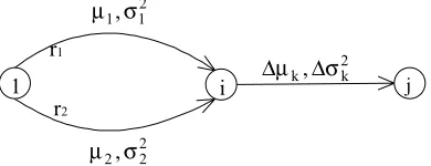
1 i j r1
r2
Figure 1. A PERT network with means and standard deviations for paths.
This path provides the least upper bound
estimate for
P T{ }
*≤t. Meanwhile,
assuming r
1,
r2∈R, and a project deadline t,
Soroush defines that r
1stochastically
dominates r
2, written as:
{
} {
}
r1fr2 , if p Z z≤ 1 <p Z z≤ 2 , or if z1<z2.
MCP IDENTIFICATION
In order to avoid complex integrations to compute (4), Soroush [21] establishes a domination structure between paths by which MCP is identified. Now, consider the PERT network of Figure 1.
He shows that if
r
1f
r
2 thenz
1<
z
2, but this relation will no longer hold when r1 and r2 are augmented by ∆r Letk. σ1<σ2 then,r1o∆rk fr2o∆rk if
(
)
(
)
t k t
k
k k
− +
< − +
µ σ
µ σ
1 1
2 2
∆µ ∆µ
(6) where σik =
[
σi2 + k2]
i=1 2
1 2
∆σ , ,
That is
(
)
(
)
(
)
∆µk ∆σk k k
k k
z t t
> = − − −
−
12 1 2 2 1
1 2
σ µ σ µ
σ σ (7)
where z12
(
∆σk)
, the threshold between r1 and r2when augmented by ∆rk is a function of only ∆σk
of ∆rk.
Soroush [21] identifies six properties about
(
)
z12 ∆σk and the domination between paths:
1. If µ1≥µ2, then z12
(
∆σk)
is a decreasingfunction of ∆σk.
2. If µ1<µ2, then z12
(
∆σk)
is an increasingfunction of ∆σk.
3. If µ2 < <t µ1or µ1>µ2>t, then z12
(
∆σk)
isnegative and decreases with ∆σk.
4. If property 3 holds, then (7) is satisfied for any
∆µkand ∆σk, that is r1o∆rk fr2o∆rk for any
∆σk.
5. If property 3 does not hold (7) is satisfied for: (5.1) µ1≥µ2, then r1o∆rk fr2o∆rkfor any ∆σk.
(5.2) µ1<µ2, then r1o∆rk fr2o∆rk for some
∆σk.
Remark 1 - We refer to the interval
[
z12(
∆σk)
,+∞]
, as the dominated interval of r1, because it is internal if ∆µkfalls within it, then r1 f r2.6. If property 3 and inequality (7) are not satisfied, then r2o∆rk f or1 ∆rk for some ∆rk.
Remark 2 - If r2o∆rk f or1 ∆rk for some ∆rk and the location of node vn of the network is such that
(
)
[
]
∆i ∆σ
k z k
µ ∈ 0, 12 , where ∆i k
µ is the largest expected duration of a path segment between vi and vn, then there will be no path segment that would alter the relation r2o∆rk f or1 ∆rk. Hence, r1 can be eliminated.
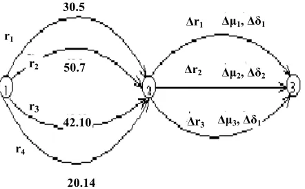
Soroush’s method to identify MCP is based on the above properties as a domination structure. Consider the network in Figure 2.
∆∆∆∆r1
∆∆∆∆r2
∆∆∆∆rn
µµµµ1 , δδδδ1
∆∆∆∆µµµµ1 , ∆∆∆∆σσσσ1
∆∆∆∆r1
∆µ ∆σk, k2
µ σ1, 12
µ σ2, 22
j 1 r2 k n
r1
rm
Figure 2. A PERT netwrok with internally disjoint paths between nodes.
1 r1 i j
r2
In Soroush’s method, for any ∆rk, the domination between r1 to rm is identified and with known ∆µk, the appropriate path that dominates
others is obtained. (This is named algorithm number 1 in Soroush’s). Therefore, there are totally n evaluations as performed in Figure 2. In Soroush’s study, the domination evaluation between r1 to rm is performed, but this evaluation is not performed about path segments
( )
∆rk . Now consider the network in Figure 3.Proposition 1 – Let σ1<σ2,∆µ1≤∆µ2,
1 2
2 1 2
1 σ ,µ µ µ µ
σ ≤∆ > > < <
∆ t or t , then in
Figure 3, r1o∆r2 is MCP if t t
−
− <
− − µ
µ
σ σ
σ σ
2 1
21 22 11 12
.
Remark 3 - This proposition means that in the mentioned case, among four paths, r1o∆r2 has smallest z.
Proof - Based on conditions in the proposition,
σ11−σ21<σ12 −σ22. Now, the condition in which
( )
(
)
z12 ∆σ1 >z12 ∆σ2 would be:
(
)
(
)
(
)
(
)
σ µ σ µ
σ σ
σ µ σ µ
σ σ
11 2 21 1
11 21
12 2 22 1
12 22
t− − t− t t
− >
− − −
−
(8) Because the two denominators of the above
relation are negative (Property 3), then we have t
t
−
− <
− − µ
µ
σ σ
σ σ
2 1
21 22 11 12
(9) If in this proposition ∆µ1>∆µ2, then from
property 3 we have
( )
(
)
∆µ1>∆µ2>z12 ∆σ1 >z12 ∆σ2 (10)
Hence, the domination of r1o∆r2 is proved.
Generalization of Proposition 1 - Let
∆σ1<∆σ2 , µ1>µ2>t or µ2< <t µ1 and σ1≤σ2
, then r1o∆r2 is MCP at Figure 3, if t
t
−
− <
− − µ
µ
σ σ
σ σ
2 1
21 22 11 12
.
Remark 4 – (i) Let σi <σj and ∆σ1<∆σ2 <...., if
µj< <t µi, then based on property 3 and
generalization of proposition 1, the condition t
t
j i
jk jk ik ik
−
− <
− −
′ ′
µ µ
σ σ
σ σ is satisfied for any
{
1,....,n}
k , k
k
k<′′∈ . In this case
t t
j i
− − µ
µ is negative and
the right-hand-side of the relation is positive, then ri rm
m ko< ′∆
is dominated, although in Soroush’s domination structure only rjo∆rk is dominated. (ii) Let σi<σj , ∆σ1<∆σ2 <...., if µi>µj>t,
the condition of t t
j i
jk jk ik ik
−
− <
− −
′ ′
µ µ
σ σ
σ σ , where
{
}
k k n
k k,< ′′ ∈1,..., should be checked and if satisfied,
then rio∆rk′ is MCP among four paths rio∆rk , rio∆rk′, rjo∆rk , rjo∆rk′. But based on Soroush’s domination structure only rio∆rk dominates others. Soroush provides algorithm number 2 to identify MCP in networks as Figure 2 shows. Based on proposition 1, this algorithm is developed.
DEVELOPEMENT OF SOROUSH’S ALGORITHM NUMBER 2 TO IDENTIFY
MCP IN NETWORK FIGURE 2
Step 1 - (Indexing and arranging)
(i) Index ri , i = 1, .... , m, such that
σ1<σ2 < <... σm.
(ii) Arrange µi,i=1,..., ,m and deadline t in
ascending order.
µi1<µi2 < <... µij < <t µij+1 < <... µim (11)
(iii) Index ∆r kk, =1,...,n, such that
∆σ1>∆σ2 > >... ∆σn.
Step 2 – (i) Consider the paths, which satisfy the conditions µj< <t µiandµi >µj>t.
(ii) Consider the paths, which satisfy the condition µj< <t µi, then proposition 1 is checked so that ri would not be eliminated later.
Step 3 - Consider the indices i1... im given by (11) in turn and eliminate the dominated path
rik(Property 4) if its index ik, k∈
{
1,...j}
is larger than some il that appear later in the order ij+1...im. Similarly, eliminate the dominated path rikif its index{
}
later in the order ij+1... im.
Step 4
– (
i) If only rm remains, terminate; rm o∆r kk, =1,...,n (except those are dominated at Step 2) are the candidates for the MCP.(ii) If more than one path remains, for any
∆r kk, =1,.... ,n identify the path which dominates others (in Step 3, consider results of Step 2).
Step 5 - Calculate z for any candidate constructed in previous step. The smallest z identifies MCP. In this algorithm only one condition
(
µj < <t µ σi, i <σj)
of proposition 1 is used. IfStep 2 is developed by merging other conditions
(
µi >µj>t,σi <σj)
, better results are obtained.In the following Example 1 is presented to demonstrate how the improved algorithm of Soroush works and reflects the difference in the manner of implementation of the new method and that on Soroush's.
Example 1 - Consider PERT network in Figure 4, Let t = 35 and
∆
σ
1=
8
,
∆
σ
2=
6
,
∆
σ
3=
3
, then µ4<µ1< <t µ3<µ2 and based on Property 4,r3 and r4 are eliminated later. For domination about ∆rk, one case should be considered:
, ,
, 2 4 1 2
2
4 µ σ σ µ µ
µ <t< where < although <t<
then
butσ <1 σ2, proposition 1 does not hold.
Consider ∆ ∆r1, r2 where ∆σ1>∆σ2. From
proposition 2, t t
−
− <
− − µ
µ
σ σ
σ σ
4 2
41 42 21 22
. Then r2o∆r2 at
∆
r2 stage evaluation andr
2o
∆
r
3at
∆
r
3stage will be eliminated. After this evaluation, r3 and r4 are eliminated. Hence, for ∆r kk, =1 2 3, , the remainderpaths are:
(i) ∆r r1 1; o∆r1 and r2 o∆r1 will be evaluated. (ii) ∆r r2; 2o∆r2 remains (at Soroush’s two paths
r1o∆r2 and r2o∆r2 remain).
(iii) ∆r r3; 1o∆r3 remains (at Soroush’s two paths r1o∆r3 and r2o∆r3 remain).
IDENTIFYING MCP IN GENERAL CASE
Based on the domination structure, a labeling algorithm for general case is presented.
Labeling Algorithm to Identify MCP in a
PERT Network
In this section a simple labeling algorithm based on the domination structure is derived that identifies MCP from the starting node to any node. Any label contains three elements. For instance the label of node vi is written as; (µi,∆σi,j), where µiandσi are themean and standard deviation of MCP to vi and j is the number of a node that vi has been labeled from it. Label of starting node is (0, 0, -). Node vi should be labeled when all nodes connected to vi have been labeled before.
Step 1 - Labeling starting node.
Step 2 - Use the CPM or a longest path algorithm to determine the largest mean duration
∆
iµ
of apath segment between each node vi, i = 2, ... ,n. Step 3 - (Labeling node vi)
Consider the nodes i1 to im which are connected to vi. They are labeled before. So, we have m paths ending to node i. Then m nodes connected to vi have labels as
(
µ σik, ik,jik)
, where k = 1,..., m andfor m paths to vi,
µk =µik + ′µk σk =
[
σik +σk]
k= m 2 2 12 , 1,..., (12)where µkand σk are the mean duration and
Figure 4. A PERT network. The two numbers beside each activity denote the expected duration and standard deviation of the activity.
r1
r2
r3
r4
30.5
50.7
42.10
20.14
∆r1
∆r2
∆r3
∆µ1, ∆δ1
∆µ2, ∆δ2
standard deviation of paths rk to vi respectively. Apply previous algorithm (Development of Soroush’s algorithm).
For MCP identification to vi, use ∆iµ. If rikdominates other paths, then label of vi would be
(
)
µik +µk σik +σk ik
, 2 2 ,
1
2 (13)
This procedure continues until vn takes a label. Remark 5 - From the third element of vn label and backward movement from the ending node to the first node, MCP will be identified.
At this stage the algorithm is complete to find MCP. The following example is presented to illustrate the matter and to show how the algorithm
works.
Example 2 - Consider PERT network in Figure 5;
∆2µ=315. ∆3µ=26 ∆4µ=16 ∆5µ=20 5.
∆6µ=10 ∆7µ=12 5. ∆8µ=5 ∆9µ=6 5.
Suppose the objective is MCP identification at t = 32. Label of v2 is (3,0.775,1) because this node has only one entry of v1. Identification of v3 label:
( )
z12 ∆σ =1 26 074. , ∆3µ>26 074. and∆3µ∈
[
0 26 074, .]
Based on Property 6, r2o∆rk dominates other paths for any ∆r kk, =1 2, and then v3 is labeled from v2 as (9, 1.817,2). Labels for other nodes would be
(
) (
)
(
)
(
) (
) (
)
(
34
.
5
,
2
.
07
,
8
)
.
:
,
7
,
1
,
26
:
,
3
,
95
.
1
,
5
.
29
:
,
2
,
9495
.
0
,
20
:
,
:
,
2
,
832
.
0
,
12
:
,
2
,
302
.
2
,
5
.
8
:
10
9 8
7
6 5
4 24.5,3.605,4
v
v
v
v
v
v
v
MCP at t = 32 moving backward from v10 is 1-2-3-8-10 and estimation of F(t) based on (4) is 0.1151.
The algorithm presented in this section recognizes the most critical path using the dominance structure. The authors of this paper provide the possibility of omitting of some other paths during the labeling process of algorithm (recognition of MCP). This possibility is made through the addition of some new conditions for the dominance structure constructed by Soroush. In fact, the domain of dominance structure is
2 5 7
4 6
1 10
3 8
9
9,0.1 8,0.2
20.5,0.5
5,0.5 10,15 0,0 0,0 0,0
4,1
15.5,4.7 6,2.7
3,0.6
7,1 18,3
10,9
10.5,1.5 6,7.7
6,0.1
6.5,0.2
4.5,0.5
Figure 5. A PERT network [21]. The two numbers beside each activity denote the expected duration and standard deviation of the activity.
3, 0.77
9, 0.32
6, 0.32
6.5,0.45 6,1.64 15.5, 2.17
4.5, 0.71
10, 3.87 6, 2.77
18,1.7
10, 3
20.5, 0.71
5, 0.71 10.5, 1.22
3 1
2 (0,0,1)
(3,0.775,1)
7,1
6,2.7
Figure 6. Labeling of node 3. 6, 1.64
extended.
NEW ESTIMATION OF F(t) BASED ON MCP DEFINITION
To estimate F(t), relation (4) is written as:
≤ ≤ ≠ ∀ ≤ ≤ ≤ ≤ = ≤ t i T p t j T j ,i k , k ,t i T , t k T p . t j T p . t i T p t * T p (14) The ratio located in the right-hand-side of (14) may be greater or smaller than one. Then we have
{
T
t
}
p
{
T
t
}
.
p
{
T
t
}
p
*≤
>
< i≤
j≤
= (15)
Based on MCP definition, ri is the path that
{
T
t
}
p
i≤
is smallest of all. Therefore;{
T
t
}
[
p
{
T
t
}
,
1
]
p
j≤
∈
i≤
(16)The path rj∈R is selected such that
{
T
t
}
p
i≤
p
{
T
j≤
t
}
provides a new estimation of F(t).Let ti>ti-1 and i 1 i i
MCP
MCP
∆
=
−, where MCPi is estimation of F(t) with MCP method at ti. Also,
{
T
t
}
p
.
MCP
MCP
* i ji
=
≤
(17)where MCPi* is a new estimation of F(t) at t
i. In order to preserve
∆
iamount as a maximum increase for estimation from ti-1 to ti we should have: i * 1 i * iMCP
MCP
∆
≤
− (18)Also MCP MCP i i * * −1
is greater than one. Then;
i * 1 i * i
MCP
MCP
1
<
≤
∆
− (19)
{
}
i * 1 i j iMCP
t
T
p
MCP
1
<
⋅
≤
≤
∆
−
(20)
{ }
T t aP a 1
j≤ ≤∆
< (21)
where ai = *
1 i i
MCP
MCP
−Relation 2.1 determines a domain through which the j-th path can be selected. This path can be beneficial to construct a new estimate of F(t) with the help of
MCP
i*. But the main attention in the design of algorithm of this section is strictly the selection of j-th path in relation 2.1 in such a way that it would be in the nearest distance to upper bound; namelyi i
a
∆
. In other words, it wouldbe more desirable than the paths are selected for which P
{ }
Tj≤t ≥0.9.Remark 6 - MCP* estimates F(t) and does not provide a bound for it.
Proof - Based on relation 2.1, we have
{
}
i1 i* 1 i i i * 1 i MCP . MCP MCP . MCP j MCP
MCP
p
T
t
− −
−
<
≤
<
(22){ }
MCP iMCP j
i *
1
i
MCP
.
p
T
t
.
MCP
MCP
1 i * 1 i − −<
≤
<
− i MCP MCP ii
MCP
MCP
MCP
i i.
1 * 1 * *1
<
<
−−− (24)
According to the definition
1
1 * 1<
− − i i MCPMCP and the inequality of the left hand side, namely
* *
1 i
i
MCP
MCP
−<
, also holds true; according to the definition of probability distribution. So we have1
b
,
bMCP
MCP
* ii
<
<
(25)where 1 * 1 − −
=
iiMCP MCP
b
. We know that F(t)<MCPi. But, in general, the kind of relation between bMCPi and F(t) is unknown. In other word, depending on b, F(t) may be less than or greater than bMCPi .So, F(t) is estimated by the appropriate determination of j-th path andp
{
T
j≤
t
}
.Approximation Algorithm for Estimating
F(t)
Step 1 - Compute F(t) for all values of t; with the help of MCP and using algorithm explained in section 5.
Step 2 - Compute
∆
ifor any ti. For the first t,∆
i should not be computed.Step 3 - Consider the first estimation (MCPi* being
equal to MCPi) and for the next ti recognize a path in the network by means of (21) and compute
MCPi*. To find the appropriate path (for example rj) to compute
p
{
T
j≤
t
i}
and to gain MCPi*, thefollowing instruction is presented.
The Instruction to Find the Appropriate
Path to Determine
p{{{{
Tj ≤≤≤≤ti}}}}
for
MCPi*Computation
Step 1 - Compute (21). (Show the resulting
interval in the form of (a, b)).
Step 2 - If for all zkn, k = 1,..., l,
p
{
z
≤
z
kn}
>
b
, finding a path that its probability at ti locates in (a,b) interval would be impossible. Then MCPi* = MCPi. Step 3 - If for all zkn, k = 1,..., l,
p
{
z
≤
z
kn}
< a ,there is a chance to find a path that its probability comes in (a, b). Here, two strategies are proposed: (i) Ignore to find a path whose probability comes in (a,b) and MCPi* = MCP
i.
(ii) Name the greatest zkn, k = 1, ..., l as zhn and the node before the last node of network that zhn was computed via it, h. Other paths from h to the last node (if exist) give probability more than zhn. If appropriate path is found, use it. Otherwise;
MCPi* = MCP
i or take another zhn which is at the nearest distance to zhn and repeat this step.
Step 4 - If for all zkn, k = 1, ..., l one or some rj are found whose probability come in (a, b) two strategies are proposed:
(i) Select the greatest zkn and compute MCPi* .
(ii) After the greatest zkn (i. e. z h n) is found, paths
which are joined to node h should be recognized and their z should be computed and if they come at (a,b) the most appropriate path should be chosen.
NUMERICAL ANALYSIS
In this section some problems to evaluate new estimation of F(t) are presented. Totally seven- problems are defined as;
(i) Two problems of Dodin’s[5] are selected. In the first problem each activity is exponentially distributed with λ= 1.5 and in the second problem each activity has the realizations 1,2,3,4,5 each with probability 0.2.
(ii) One problem of Ringer’s [2] is selected and F(t) is calculated analytically. Each activity is distributed normally or exponentially.
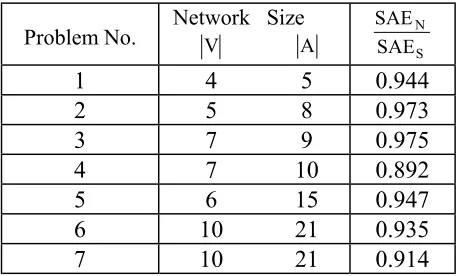
(iii) Four problems are selected from Fatemi Ghomi’s work [22], that all activities are defined by discrete random variables. In these problems F(t) are computed by means of simulation. Table 1 shows the results for the above-mentioned problems. Column 4 shows SAE
SAE
N S
, where SAEN is
the sum of absolute errors of new estimation of F(t) and SAES is the sum of absolute errors of
Soroush’s estimation of F(t) at a given time. The results indicate that the new method TABLE 1. Comparison of New Estimation and Soroush’s
to Approximate F(t) Approximation.
Problem No. Network V Size A
SAE SAE
N S
1 4
5
0.944
2 5
8
0.973
3 7
9
0.975
4 7
10
0.892
5 6
15
0.947
6 10
21
0.935
provides better estimation than that of Soroush’s. Meanwhile, the error ratio does not prevail a significant relation between the magnitude of the error and network size. The major factor in error reduction corresponding to the new method is that it uses two paths to estimate F(t). The initial estimate of the new method is made with the help of Soroush’s algorithm. Based on this reason and (21), column 4 represents numbers completely close to one. For those networks having large number of paths, the new method has the increased chance to obtain good results. Soroush’s method provides an upper bound for F(t), but the new method does not have this property. In four problems of Table 1, for some amount of time, the new method provides smaller estimation for F(t). Usually at small amount of time, a large amount for ∆ is obtained, then (21) represents a large interval. In this case, it is probable to obtain a path to compute MCP*. When the initial estimate of new method has the value between 0.9 to 1 for F(t), if a path is found at (21), small variation occurs in the recent computation. This indicates that the new method has suitable performance. Also, when F(t) has a small amount, by obtaining large ∆, the possibility to find appropriate path at (21) increases. These points were led to derive (21).
CONCLUSION
In this paper, the purpose was MCP identification and to estimate completion time distribution function of a PERT network. A labeling algorithm is derived that acts as a simple mechanism to identify MCP from the starting node to any node in the network. An estimation method for direct computation of F(t) is presented that gives satisfactory answers in comparison with those of Soroush's.
REFERENCES
1. Harthley, H. O. and Wortham, A. W., “A Statistical Theory for PERT Critical Path Analysis”, Management
Science, Vol. 12, No.10, (1966), 469-481.
2. Ringer, L. J., “Numerical Operators for Statistical PERT Critical Path Analysis”, Management Science, Vol. 16,
No. 2, (1969), 136-143.
3. Kulkarni, V. G. and Adlakha, V. G., “Markov and Markov Regenerative PERT Network”, Journal of Operations
Research, Vol.34, No. 5, (1980), 769-781.
4. Martin, J. J., “Distribution of the Time Through a Directed, Acyclic Network”, Operations Research, Vol. 13, No.1, (1965), 46-66.
5. Dodin, B. M., “Bounding the Project Completion Time Distribution in PERT Network”, Journal of Operations
Research, Vol. 33, No. 4, (1985), 826-881.
6. Vobill, P. and Trahan, M., “The Completion Time of PERT Network”, Journal of Operations Research, Vol. 25, No. 1, (1977), 15-29.
7. Kleindorfer, G. B., “Bounding Distributions for a Stochastic Acyclic Network”, Journal of Operations
Research, Vol. 19, No. 7, (1977), 1586 - 1601.
8. Van Slyke, R. M., “Monte Carlo Methods and the PERT Problem” Operations Research, Vol. 11, No. 5, (1963), 839-860.
9. Sculli, D., “The Completion Times of PERT Network”,
Journal of the Operational Research Society, Vol. 34,
No 2, (1983), 155-158.
10. Kamburowski, J., “An Upper Bound on the Expected Completion Time of PERT Network”, European Journal
of Operational Research Society, Vol. 21, No. 2, (1985),
206-212.
11. Fulkerson, D. R., “Expected Critical Path Length in PERT Network”, Operations Research, Vol. 10, No. 6, (1962), 808-817. 12. Clingen, C. T., “A Modification of Fulkerson’s PERT
Algorithm”, Operations Research, Vol. 12, No.4, (1964), 629-632.
13. Elmaghraby, S. E., “On the Expected Duration of PERT Type Network”, Management Science, Vol. 13, No.5, (1967), 299-306.
14. Robillard, P. and Trahan, M., “Expected Completion in Time.in Part Network”, Operation Research, Vol. 24, No. 1, (1976), 177-182.
15. Lindsey, J. H., “An Estimate of Expected Critical Path Length in PERT Network”, Journal of Operations
Research, Vol. 20, No.4, (1972), 800-812.
16. Dodin, B. M., “Approximating the Distribution Function in Stochastic Network”, Computers and Operations
Research, Vol. 12, No.3, (1985), 251-264.
17. Sigal, C. E., Pritsker, A. A. B. and Solberg, J. J., “The Use of Cutsets in Monte Carlo Analysis of Stochastic Network”, Mathematics and Computers in Simulation, Vol. 21, (1979), 376-384.
18. Fisher, D. L., Saisi, D. and Goldstein, W. M., “Stochastic PERT Networks: OP Diagrams, Critical Paths and the Project Completion Time”, Computers and Operations
Research, Vol. 12, No.5, (1985), 471-482.
19. Dodin, B. and Elmaghraby, S. E., “Approximating the Criticality Indices of the Activities in PERT Networks”,
Management Science, Vol. 31, No. 2, (1985), 207-223.
20. Dodin, B. M., “Determining the K Most Critical Paths in PERT Network”, Operations Research, Vol. 32, No. 4, (1984), 859-877.
Society, Vol. 45, No. 3, (1994), 287-300.
22. Fatemi Ghomi, S. M. T., Hashemin, S. S., Teimouri, E., and Jolai Ghazvini, F., “Developing the Approaches to Compute
![Figure 5. A PERT network [21]. The two numbers beside each activity denote the expected duration and standard deviation of the activity](https://thumb-us.123doks.com/thumbv2/123dok_us/245303.2019235/6.595.62.267.564.688/figure-network-activity-expected-duration-standard-deviation-activity.webp)