The Thirty-Third AAAI Conference on Artificial Intelligence (AAAI-19)
Deep Neural Network Quantization via
Layer-Wise Optimization Using Limited Training Data
Shangyu Chen,
1Wenya Wang,
1Sinno Jialin Pan
1 1Nanyang Technological University[email protected], [email protected], [email protected]
Abstract
The advancement of deep models poses great challenges to real-world deployment because of the limited computational ability and storage space on edge devices. To solve this prob-lem, existing works have made progress to prune or quantize deep models. However, most existing methods rely heavily on a supervised training process to achieve satisfactory perfor-mance, acquiring large amount of labeled training data, which may not be practical for real deployment. In this paper, we propose a novel layer-wise quantization method for deep neu-ral networks, which only requires limited training data (1% of original dataset). Specifically, we formulate parameters quan-tization for each layer as a discrete optimization problem, and solve it using Alternative Direction Method of Multipli-ers (ADMM), which gives an efficient closed-form solution. We prove that the final performance drop after quantization is bounded by a linear combination of the reconstructed errors caused at each layer. Based on the proved theorem, we pro-pose an algorithm to quantize a deep neural network layer by layer with an additional weights update step to minimize the final error. Extensive experiments on benchmark deep mod-els are conducted to demonstrate the effectiveness of our pro-posed method using 1% of CIFAR10 and ImageNet datasets. Codes are available in: https://github.com/csyhhu/L-DNQ
Introduction
Deep neural networks have been extensively employed with promising results in various applications especially in com-puter vision (Krizhevsky, Sutskever, and Hinton 2012; Si-monyan and Zisserman 2014; He et al. 2016). However, high performance comes with huge cost brought by enor-mous amount of parameters and tremendous computational cost. Consider a very deep model which is fully well-trained and deployed, to use it for making predictions, most of the computations involve multiplications of a real-valued weight by a real-valued activation in forward propagation. These multiplications are expensive as they are all float-point to float-point multiplication operations. To alleviate this prob-lem, a number of approaches have been proposed to com-press deep models by pruning or quantization. Han et al. (2015) proposed to sparsify weights to reduce the number of multiplications directly. Courbariaux, Bengio, and David
Copyright c2019, Association for the Advancement of Artificial Intelligence (www.aaai.org). All rights reserved.
(2015) and Hubara et al. (2016) proposed to binarize weights to be in{±1}. Rastegari et al. (2016) introduced a float value αlknown as thescaling factorin layerl, turning binarized weights asαl× {±1}. To accelerate inference,αlis multi-plied by layer input, such that weights become integer values
{±1}, converting float-point multiplication into float-point to integer computation. Li, Zhang, and Liu (2016) extended binary weights to ternary values, and Leng et al. (2017) fur-ther proposed to quantize the models with more bits in or-der to provide more flexibility. Apart from above mentioned training-based method, direct quantization methods also ex-ist that don’t require training data: Gong et al. (2014) clus-tered weights using Kmeans. Jacob et al. (2017), Vanhoucke, Senior, and Mao (2011) projected weights to nearest dis-crete points. Li et al. (2017) proposed convergence analysis of quantization training.
However, most prevailing low bits compression methods relied on a heavy training process with large amount of la-beled data. Specifically, given a pre-trained full-precision deep neural network as the initial parameters, which is usu-ally trained in a cloud environment, most methods carry the compression process in a supervised learning manner with sufficient training data by minimizing the error between the compressed network outputs and the ground-truth labels. However, practical scenarios pose more strict challenges. On the one hand, excessive training data for a specific applica-tion is inaccessible due to data privacy, especially in com-mercial models with high confidential requirement (Wu et al. 2016). On the other hand, many real cases require the com-pression conducted on edge devices, which greatly limit the storage space to deploy large amount of training data (e.g. ImageNet dataset occupies over 500Gb). Therefore, com-pression underlimited instancesis crucial in practice.
the original full-precision parameters. 2) The quantization can be obtained in a closed-form solution without gradient-based training. 3) There is a theoretical guarantee on the overall prediction performance after quantization. 4) The whole process consumes only a small portion of instances from training data (1% of training dataset in experiments).
To achieve the first goal, we formulate a quadratic opti-mization problem for each layer to minimize the error be-tween the quantized layer output and the full-precision layer output. The quantized weights serve as discrete constraints, leading to a discrete optimization problem. This problem is solved by Alternative Direction Methods of Multipliers (ADMM) (Boyd et al. 2011) that decouples the continuous variables and discrete constraints to update them separately. ADMM is highly efficient and provides a closed-form so-lution to our quantization problem which contributes to our second goal. Regarding our third goal, inspired by (Aghasi et al. 2017; Dong, Chen, and Pan 2017) which provide theoret-ical bounds for network pruning, we derive a bound for net-work quantization. Most importantly, to avoid inefficient us-age of data as is common in existing works, we approximate full-precision network under quantized constraints without the need for label supervision for optimization except a light retraining process. Experiments verify that the quantized networks learned by our proposed method with limited train-ing data only brtrain-ing a slight drop of the prediction perfor-mance, which achieves our fourth goal.
L-DNQ is able to achieve promising results with only limited training data compared with existing quantization methods. In practice, L-DNQ shows tremendous efficiency in data usage compared with some state-of-the-art methods.
Related Work
Regarding deep networks quantization, Courbariaux, Ben-gio, and David (2015) proposed network binarization through deterministic and stochastic rounding for parame-ters update after backpropagation. Hubara et al. (2016) and Rastegari et al. (2016) extended the idea by introducing bi-nary activation. However, they all fail to recover a closing accuracy of the full-precision models. Li, Zhang, and Liu (2016) assumed a prior distribution for parameters to find an approximated threshold for ternarization. However, a proper prior is difficult to define. Lin, Zhao, and Pan (2017) ap-proximated the full-precision weight with a linear combi-nation of multiple binary weight bases. Zhu et al. (2016) set different scaling factors for positive and negative param-eters ternarization. To update these factors, they first per-formed gradient descent, then gathered and averaged gradi-ents for different factors based on some heuristic thresholds. Both of these methods relied on retraining and manually de-signed thresholds. Leng et al. (2017) modified the quanti-zation retraining objective function using ADMM, which separates the processes on training real-valued parameters and quantizing the updated parameters. Zhou et al. (2017) proposed to incrementally quantize a portion of parame-ters based on weight partition. Polino, Pascanu, and Alis-tarh (2018) used distillation to assist training quantized net-work. All the above approaches relied on heavy supervised training process. Hou and Kwok (2018) extended neural
network binarization from (Hou, Yao, and Kwok 2016) to quantization. By directly quantizing weights without train-ing, Gong et al. (2014) clustered weights using Kmeans, Ja-cob et al. (2017), Vanhoucke, Senior, and Mao (2011) pro-jected weights to nearest discrete points, Kundu et al. (2017) approximated full-precision weights by addition of a set of discrete values. Lin, Talathi, and Annapureddy (2016) con-verted pre-trained floating point models based on ignal-to-quantization-noise-ratio (SQNR). Still, such direct quantiza-tion can hardly cover performance drop. Other related works to ours include (Aghasi et al. 2017) and (Dong, Chen, and Pan 2017), which are also layer-wise deep compression ap-proaches. However, they focused on pruning unimportant weights of the original networks rather than quantizing the real values of the weights into discrete bits.
Problem Statement and Preliminary
Problem Statement
Given a training set of n instances of d dimensions,
{xj, yj}nj=1, and a well-trained deep neural network with
Llayers (excluding the input layer)1. The well-trained
net-work is considered as a reference or teaching netnet-work. De-note the input and the final output of the well-trained deep neural network byX= [x1, ...,xn]∈Rd×nandY∈RmL×n,
respectively. For a layerl, we denote the input and the out-put of the layer byYl−1= [yl−1
1 , ...,yln−1]∈Rml−1×nand
Yl= [yl
1, ...,yln]∈Rml×n, respectively, where yli can be considered as a representation ofxiin layerl, andY0=X,
YL = Y,m
0 = d. Using one forward-pass step, we have
Yl=σ(Zl), whereZl=W¯>l Yl−1withW¯l∈Rml−1×ml
denoting the matrix of full-precision parameters for layerl of the well-trained neural network, andσ(·)is the activation function. For convenience in presentation and proof, we de-fine the activation function σ(·)as the rectified linear unit (ReLU). We further denote by Θ¯l ∈Rml−1ml×1 the vec-torization ofW¯l. For a well-trained neural network,Yl,Zl andΘ¯lare all fixed matrices and contain most information of the neural network. The goal of quantization is to dis-cretize the values of all elements ofΘ¯lfor each layer into a finite setΩl, e.g. symmetric:Ωl={−αl,0, αl}or random:
Ωl={αl, βl, γl}. We denote the quantizedΘ¯lbyΘˆl.
Alternative Direction Methods of Multipliers
ADMM is a widely-used optimization method (Aghasi et al. 2017; Takapoui et al. 2017). It combines the decomposabil-ity of dual ascent and convergence properties of the methods of multipliers. Given the following minimization problem:
minf(x) +g(z), s.t.h(x,z) =0.
In ADMM, we first reformulate (1) with augmented La-grangian as:
Lρ(x,y,z) =f(x)+g(z)+y>h(x,z)+ρ
2||h(x,z)||
2 2, (1)
1
whereyis the Lagrangian multipliers. In practice,yis re-placed byλ= (1ρ)y(Boyd et al. 2011) to convert (1) to
Lρ(x,y,z) =f(x)+g(z)+ ρ
2||h(x,z)+λ||
2 2−
ρ 2||λ||
2. (2)
We then breaks (2) into subproblems with respect tox,z, λ, respectively, and solve them iteratively using the following updates:
Proximal step:xk+1=argmaxxLρ(x,zk,λk) (3) Projection step:zk+1=argmaxzLρ(xk+1,z,λk)(4) Dual update Step:λk+1=λk+xk+1−zk+1 (5)
Layer-Wise Quantization
Our proposed L-DNQ is a layer-wise cascade algorithm, where the output of a quantized layer is used as the input for quantizing the subsequent layer. Specifically, suppose one has quantized the well-trained network up to the(l−1)-th layer. Then, to quantize thel-th layer, we considerYˆl−1 =
f(Y0;Θˆ[1,...,l−1]) as the input, where f(Y0;Θˆ[1,...,l−1])
denotes the output of the (l−1)-th layer with the first (l−1) layers being quantized, given input Y0. In the subsequent steps, L-DNQ aims at quantize the weights from layerlto the last layer L, denoted byΘˆ[l,...,L], such that the
diver-gence of the final layer output between quantized network and pre-trained network is minimized:
min ˆ Θ[l,...,L]
||f(Yˆl−1;Θˆ[l,...,L])−f(Yl−1;Θ¯[l,...,L])||2F,(6)
s.t. Θˆ[l,...,L]∈Ω[l,...,L].
Directly solving the above problem is difficult as the in-puts to quantized network (Yˆl−1) and the reference network
(Yl−1) are different. Here, instead we propose to optimize the upper bound of the objective in (6), which is given by the following triangle inequality:
||f(Yˆl−1;Θˆ[l,...,L])−f(Yl−1;Θ¯[l,...,L])||2F
≤ ||f(Yˆl−1;Θˆ[l,...,L])−f(Yˆl−1;Θ¯
new
[l,...,L])|| 2
F
| {z }
Quantization
+||f(Yˆl−1;Θ¯new[l,...,L])−f(Yl−1;Θ¯[l,...,L])||2F
| {z }
Weights Update
,(7)
where f(Yˆl−1;Θˆ
[l,...,L]) presents the final output with
quantized weightsΘˆ[l,...,L] and inputYˆl−1.Θ¯
new
[l,...,L] is
in-troduced as updated full precision weights learned during training. The objective in (6) is upper bounded by the sum-mation of theQuantizationterm and theWeights Update term. To optimize its upper bound, we present an ADMM algorithm to minimize the Quantization term for each layer and a back-propagation algorithm to minimize the Weights Update term right after the quantization on each layer. These two procedures are conducted alternatingly until all layers are quantized.
Layer-Wise Error
During layer-wise quantization in layerl, which is the quan-tization term in (7), supposeΘˆlis the quantized parameters ofΘ¯newl (whenl= 1,Θ¯1new=Θ¯1; matrix form asW¯newl ) to be learned. With the cascade inputYˆl−1andΘˆl, we ob-tain a new outcome of the weighted sum before performing the activation functionσ(·)for layerl, denoted byZˆl. Com-pared with the weighted sum of updated weights and cascade input: Zl
∗ = (W¯newl )>Yˆl−1, we define an error function E(·)as:
El=E(Zˆl) = 1 n
ˆ Zl−Zl∗
2
F, (8)
wherek · kF is the Frobenius Norm. Based on the definition of the error function (8), E(Zl∗) = 1nZl∗−Zl∗
2
F = 0. Using this property and following (Hassibi and Stork 1993; LeCun, Denker, and Solla 1990), (8) can be approximated by functional Taylor series as follows,
El=E(Zˆl)−E(Zl∗) (9)
=
∂El
∂Θl
>
δΘl+ 1 2δΘl
>H
lδΘl+O(kδΘlk32),
where δΘl denotes a perturbation of Θ¯ new
l , Hl ≡ ∂2El/∂Θl2is the Hessian matrix w.r.t.Θl. It can be proven that with the error function defined in (8), the first (linear)
term ∂∂EΘl
l
Θl=Θ¯newl = 0, andO(kδΘlk
3
2)vanishes. Hence
we can rewrite (9) asEl= 12δΘl>HlδΘl. Since our goal is to quantize the weights to obtainΘˆ, by replacingδΘlwith
ˆ Θl−Θ¯
new
l , the final objective becomes:
min ˆ Θl
f(Θˆl) = 12(Θˆl−Θ¯ new
l )>Hl(Θˆl−Θ¯ new l ), (10)
s.t. Θˆl∈Ωl,
whereΩlis a discrete set of all possible values of the quan-tized weights in layerl. To solve (10), which is a discrete op-timization problem, we develop a ADMM-based algorithm.
Quantization with ADMM
In our problem setting, we apply ADMM to separately op-timize continuous variables and discrete variables in (10). To be specific, we introduce an auxiliary parameterGand reformulate (10) as follows,
min ˆ Θ,G
f(Θˆ) +IΩ(G), s.t. Θˆ =G, (11)
where IΩ(G) is an indicator function that induces great penalty ifG 6∈ Ω. Here we drop the subscript l for sim-plification in presentation. By introducing Gand applying the ADMM algorithm, the optimization problem (11) can be converted to
Lρ(Θˆ,G,λ)
=f(Θˆ) +IΩ(G) +
ρ 2k
ˆ
Θ−G+λk2 2−
ρ 2kλk
2 2.(12)
Proximal Step At iteration k+ 1, the proximal step in-volves the update onΘˆ via
ˆ
Θk+1=argmin ˆ Θ
Lρ(Θˆ,Gk,λk), (13)
where
Lρ(Θˆ,Gk,λk) =f(Θˆ) +ρ 2k
ˆ
Θ−Gk+λkk2
2. (14)
Sincef(Θˆ)is a quadric function with continuous variable, setting the gradient to 0 leads to the optimal solution by solving the following linear equation:
H+diag(ρ)Θˆk+1=H ¯Θnew+diag(ρ)(Gk−λk). (15)
This is far more efficient than gradient descent (Leng et al. 2017), and costs only a few seconds even if H is large. Besides, gradient descent requires fine-tuning a number of hyper-parameters and has unpredictable convergence. These issues are avoided using (15). As we can observe in (14),ρ acts as an importance weight for the discrete term. A largeρ
leadsΘˆk+1to approach discrete feasible solutionGk−λk, while a smallρguides it to original weightsΘ¯new.
Projection Step In projection step, we optimize G by solving the following optimization problem:
min
G k
ˆ
Θk+1−G+λkk2
2, s.t. G∈Ω. (16)
We defineVk =Θˆk+1+λk, which is fixed in the projec-tion step. The goal of (16) is to findGthat is closest toVk and lie in the discrete setΩ. TakeΩ = {−α,0, α} as an example. We further denote byQ∈ {−1,0,1}an interme-diate variable such thatG = g(α,Q) = α·Q. Hereg(·) represents a mapping from integers to discrete real values. Thus, (16) can be rewritten as:
min G,αkV
k−α·Qk2
2, s.t. Q∈ {−1,0,1}, (17)
which consists of two types of variables to be optimized: the scaling factorαthat is continuous and the discrete con-straints Q. The problem is non-convex and non-smooth. We propose to solve it alternatingly: optimize α with Q
fixed and vice versa. Specifically, given a fixed Q, (17) is a quadric function w.r.t α, which can be easily solved by α = VQ>>QQ. With α fixed, the optimal Q is obtained
by projecting Vk to the nearest feasible solution as Q =
Proj{−1,0,1}
Vk α
, where ProjΩ(x) denotes the nearest point in the setΩ forx. The projection step is efficient to compute. Empirical experiments show thatαandQcould reach a stable range in less than 10 iterations. Finally we can haveGk+1=g(α,Q).
Dual Update Step After obtainingΘˆk+1andGk+1, the dual variableλis updated using the following rule:
λk+1=λk+Θˆk+1−Gk+1. (18) The ADMM-based layer-wise optimization saves much effort compared to existing gradient-descent-based meth-ods. Computation complexity for the three steps are:
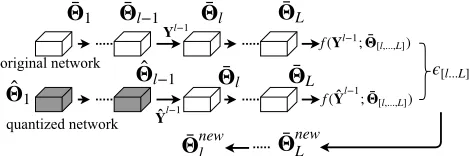
quantized network original network
Figure 1: Weights Update: After layer l − 1 is quan-tized from Θ¯l−1 to Θˆl−1. Input Yl−1 and Yˆl−1 are
fed into two networks to generate f(Yl−1;Θ¯[l,...,L]) and
f(Yˆl−1;Θ¯
[l,...,L]), respectively. Squared difference is
back-propated to update weights in higher layers:Θ¯newl,...,L.
O(n3),O(n),O(n), where n is the number of weights in one
kernel. Most importantly, solving the optimization objective requires no label information, which is beneficial when la-beled data is not available in real world applications.
Remaining Non-quantized Layers Update
In order to optimize the weights update term in (7), we first obtain the network where the previousl−1layers are quantized while the remaining ones are not. Denote the dif-ference or error of the final layer output between the cur-rent partially-quantized network and the original network by [l...L] = kf(Yˆl−1;Θ¯
new
[l,...,L])−f(Yl−1;Θ¯[l,...,L])k2F. Here, we consider f(Yl−1;Θ¯
[l,...,L]) as the ground-truth,
and use back-propagation to learnΘ¯new[l,...,L]. After we update
¯
Θ[l,...,L]toΘ¯
new
[l,...,L], we can apply the ADMM algorithm
in-troduced in the previous section to quantize layerlby replac-ingΘ¯l withΘ¯
new
l in (10). Fig.1 demonstrates the weights update procedure.
Algorithm 1Layer-wise Unsupervised Network Quantiza-tion
Require: Θ¯ = {Θ¯l}1≤l≤L, C = {µl, σl, γl, βl}1≤l≤L:
well-trained network,X: training data
Ensure: Θˆ = {Θˆl}1≤l≤L, Cˆ = {µˆl,ˆσl,γˆl,βˆl}1≤l≤L, {αl}1≤l≤L: quantized network
1: forl= 1,2, ...Ldo
2: Calculate Hessian matrixHl of layerl from Θ¯ new l andX. (Ifl= 1,Θ¯new1 =Θ¯1)
3: Perform ADMM to obtain quantized weightΘˆl by solving (12)
4: Learn Θ¯new[l+1,...,L] by minimizing [l+1...L] =
kf(Yˆl;Θ¯new
[l+1,...,L])−f(Yl;Θ¯[l+1,...,L])k2F, and up-dateΘ¯[l+1,...,L]←Θ¯
new
[l+1,...,L].
5: end for 6: Retrain.
L-DNQ in Practice
batch normalization, which is also updated in the quantized network. Steps 1-5 corresponds to the quantization proce-dure using ADMM. After quantization, models can be fur-ther boosted by retraining: using label information to fine-tune parameters in batch normalization layers and unquan-tized layer. In practice, we adopt approximated Hessian cal-culation in (Dong, Chen, and Pan 2017), which only needs to calculate one block matrix of the original Hessian, making our Hessian computation suitable to handle. About 200 im-ages are sufficient to generate Hessian matrix for each layer.
Theoretical Analysis
Recall that our goal is to control the consistency of the net-work’s final outputYLbefore and after quantization. In the following, we show how the layer-wise errors propagate to the final output layer. We prove that the accumulated error over multiple layers is upper bounded by a constant.
Theorem 1. Given a quantized network via layer-wise quantization introduced in Section , each layer has its own layer-wise error εlfor 1 ≤ l ≤ L, then the accumulated error of ultimate network output εˆL = √1
nkYˆ
L −YLk F
obeys:
ˆ εL≤
L−1
X
k=1
L
Y
l=k+1
A√εk
!
+√εL, (19)
whereYˆl=σ(Wˆ>
l Yˆ
l−1)for2≤l≤Ldenotes the
“accu-mulated pruned output” of layerl. The termA=kΘˆlkF is
upper bounded according to different quantizations.
ConsiderΩ={±α,0} as an example. It can be proven that A ≤α2×(ml×ml−1). Moreover, empirical
experi-ments shows that0occupies 50%-70% of the quantized pa-rameters, thusAis much smaller in practice. In summary, Theorem 1 shows that: 1) Layer-wise error for layerlwill be scaled by continued multiplication of parameters’ Frobe-nius Norm over the following layers when it propagates to final output. For quantization, this Frobenius Norm is upper bounded by a constant determined by the quantization in-tervals. 2) The final error of the ultimate network output is bounded by the weighted sum of layer-wise errors.
Proof. We prove Theorem 1 via induction. First, forl= 1:
ˆ
εl=εl=
√
δEl. (20)
Then suppose that Theorem 1 holds up to layerl:
ˆ εl≤
l−1
X
h=1
( l
Y
k=h+1
kΘˆkkF
√
δEh) +√δEl. (21)
In order to show that (21) holds for layerl+ 1as well, we refer toY˜l+1=σ(Wˆ>l+1Yl)as ‘layer-wise quantized out-put’, where the inputYl is fixed as the same as the origi-nally well-trained network. An accumulated inputYˆl+1 =
f(Y0;Θˆ[1,...,l]), and have the following theorem.
Theorem 2. Consider layer l+ 1 in a quantized deep network, the difference between its accumulated quantized
output, Yˆl+1, and layer-wise quantized output, Y˜l+1, is bounded by:
kY˜l+1−Yˆl+1k2F ≤
√
nkΘˆl+1k2Fεˆ l.
(22)
By using (20), (22) and the triangle inequality, we are now able to extend (21) to layerl+ 1:
ˆ
εl+1 = √1
nk
ˆ
Yl+1−Yl+1k2
F
≤ √1
nk
˜
Yl+1−Yˆl+1k2
F + 1
√
nk
˜
Yl+1−Yl+1k2
F
≤
l
X
h=1
l+1
Y
k=h+1
kΘˆk+1k2
F ·
√
δEh
!
+
√
δEl+1.
Finally, we prove that (21) holds up for all layers, and Theorem 1 is a special case when l = L. We further set
A = kΘˆlkF, which is the Frobenius norm of quantized weights. A is upper bounded according to different quan-tization. Consider Ω ={±α,0} as an example. It can be proven thatA ≤α2×(ml×ml−1).
Experiment
Experimental Setup
We conduct comparison experiments with the following baseline approaches: 1) Extremely Low Bit Neural Network (ExNN) (Leng et al. 2017) 2) Trained Ternary Quantization (TTQ) (Zhu et al. 2016), 3) Incremental Network Quantiza-tion (INQ) (Zhou et al. 2017) 4) Loss-Aware weight Ternar-ized network (LAT) (Hou and Kwok 2018). 5) Compress-ing Deep Convolutional Networks usCompress-ing Vector Quantiza-tion (VQ) (Gong et al. 2014). 6) Direct QuantizaQuantiza-tion (DQ) which is commonly used in production (Jacob et al. 2017), (Vanhoucke, Senior, and Mao 2011). 7) Ternary Residual Networks (TRN) (Kundu et al. 2017). 8) Model compression via distillation and quantization (DistilQuant) (Polino, Pas-canu, and Alistarh 2018). Two benchmark datasets are used including ImageNet ILSVRC-2012 and CIFAR-10. Regard-ing deep architectures, we experiment with ResNet-18 (He et al. 2016), AlexNet2 (Krizhevsky, Sutskever, and Hinton
2012) on ImageNet dataset, and with CIFARNet3, VGG, WRN4, ResNet-20, ResNet-32, ResNet-56 on CIFAR-10.
All these deep models are well trained at the first place. Due to different deep learning framework, performance of well-trained networks show slight difference.
As L-DNQ pioneers in limited-instance quantization, few works have been published for comparison. VQ conducts compression based on original pre-trained model by using K-means clustering directly; DQ essentially projects full-precision weights into nearest discrete points; TRN approx-imated full-precision weights by a combination of quan-tized weights. After quantization, training instances are used
2AlexNet with batch normalization layers is adopted. 3
The network architecture is:(2×128C3)−M P2−(2×
256C3)−M P2−(2×512C3)−M P2−(2×1024F C)−
10SV M, whereC3is a3×3ReLU convolution layer,M P2is a
2×2max-pooling layer. 4
for retraining and fine-tunning. These methods can be con-sidered as baselines for limited-instance quantization. For fair comparison with training-based quantization, we reduce training data to 1% of the original training dataset. Specif-ically, we re-implement ExNN, TTQ, INQ, LAT and Dis-tilQuant to generate their reported results and then apply the same sets of parameters to produce the results with limited instances. 500 training instances in CIFAR-10 and 12,800 in ImageNet are randomly sampled to simulate the scenario of limited instances. All experiments are conducted 5 times and the average result is reported. Note that all methods use different initial pre-trained models. For fair comparison, we record the percentage of the improvements for these quan-tized models over their corresponding pre-trained models, which is positive for improvement while negative for degra-dation after quantization (The higher the better).
L-DNQ adopts the following quantization intervals:Ωl= αl× {0,±20,±21,±22...±2b}for each layer. Using power of 2 is efficient for inference, because quantized weights can be stored and calculated as integer (±1,2, ...), with layer output multiplying by αl to retrieve the actual layer out-put. To facilitate notation, we use(2b+3)-bit to denote the above quantization set, which can be interpreted as the to-tal number of different values in the quantization set, e.g., α× {0,±20,±21,±22}is denoted as 7-bit. In INQ (Zhou
et al. 2017), (Jacob et al. 2017) and (Kundu et al. 2017), a different presentation form for bits is used. Here we convert the number of bits using our notation for fair comparison.
Network Method bits Imp∗(%) FP∗∗
ResNet20
TTQ 3 -77.25 91.77 INQ 15 -48.48 90.02 ExNN 3 -11.15
91.5 VQ 3 -11.27
DQ 3 -19.92 L-DNQ 3 -4.30
ResNet32
TTQ 3 -79.99 92.33 INQ 15 -48.02 86.83 ExNN 3 -12.03
92.13 VQ 3 -8.98
DQ 3 -21.07 L-DNQ 3 -3.66
ResNet56
TTQ 3 -80.64 93.20 INQ 15 -15.84 93.40 ExNN 3 -12.15
92.66 VQ 3 -11.43
DQ 3 -18.67 L-DNQ 3 -3.49
CIFARNet
LAT 3 -11.62 89.62 VQ 3 -11.83
92.27 DQ 3 -21.72
L-DNQ 3 -1.96
VGG∗∗∗ DistilQuant 3 -53.9 90.77 L-DNQ 3 -1.47 89.42
WRN DistilQuant 3 -6.57 92.25 L-DNQ 3 -2.22 91.43
Table 1: Comparison on CIFAR-10. All methods use 1% (500 images) of training instances.∗indicates improvement.
∗∗ representsFullPrecision (pre-trained model) Accuracy. ∗∗∗is a VGG-like model adopted by DistilQuant.
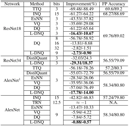
Network Method bits Improvement(%) FP Accuracy
ResNet18
TTQ 3 -69.48/-88.49 69.6/89.2
INQ 15 -61.27/-64.22 68.27/88.69
ExNN 3 -43.53/-37.82
69.76/89.02
VQ 3 -35.69/-29.08
DQ 3 -61.22/-65.64
L-DNQ 3 -16.43/-10.67
DQ
8 -56.78/-58.92 16 -13.81/-8.68 32 -2.82/-1.51
L-DNQ 9 -2.73/-0.90
ResNet34 DistilQuant 3 -32.03/24.3 56.55/79.09
L-DNQ 3 -29.31/18.37
AlexNet1
TTQ
3
-56.18/-78.26 57.2/80.3 DistilQuant -55.07/-72.79 56.55/79.09
ExNN -28.34/-26.06
58.34/80.80
VQ -35.95/-36.06
DQ -57.04/-76.49
L-DNQ -17.78/-14.00
AlexNet
INQ 15 -42.82/-46.83 57.24/79.80
TRN 12.5 ≈ −1 N.A.
ExNN
9
-13.47/-10.33
58.34/80.80
VQ -5.94/-4.22
DQ -7.84/-5.72
L-DNQ -0.88/-0.57
Table 2: Comparison on ImageNet. All methods use 1% (12,800 images) training instances. AlexNet1: in TTQ, the
weights of the first and final layer remain full precision. L-DNQ, ExNN, DQ, VQ, DistilQuant are under the same set-ting.
Overall Experimental Results and Analysis
On CIFAR-10, we compare our method with ExNN, TTQ, INQ, LAT, VQ, DQ, DistilQuant in Table 1. ExNN incorpo-rated ADMM quantization in training. TTQ ternarized the full-precision model into 3 different values: {βl,0, αl} in layerl. INQ converted weights into either power of two or zero. LAT quantized weights into 3 bits. DistilQuant utilize distillation to train quantized model. We reproduce TTQ, INQ experiments on ResNet-20, ResNet-32, ResNet-56, LAT experiments on CIFARNet and DistilQuant on VGG, WRN with the source code released by (Zhu et al. 2016) , (Zhou et al. 2017) , (Hou and Kwok 2018) and (Polino, Pascanu, and Alistarh 2018), respectively. ExNN is reim-plemented by us since its source code is not released. After VQ and DQ generate quantized weights, we use limited in-stances for retraining. As Table 1 shows, all training-based methods (ExNN, TTQ, INQ, DistilQuant) experienced great degradation using limited instances. VQ and DQ performed slightly better, but still showed considerable drop. As a con-trast, L-DNQ can preserve original performance, even under a dramatic reduction of training data down to 1%.
1 10 20 40 60 100 Instances Used (%) −80
−70 −60 −50 −40 −30 −20 −10 0
Testing Accuracy Improvement (%)
L-DNQ TTQ INQ VQ DQ ExNN
(a)
1 5 10 20 40
Instances Used (%) −70
−60 −50 −40 −30 −20
Top 1 Accuracy Improvement (%)
L-DNQ TTQ INQ VQ DQ ExNN
(b)
0 2 4 6 8 10 12 14 16 Layer Output Error 20
40 60 80 100
Testing Error(%)
Top1 Error Top5 Error
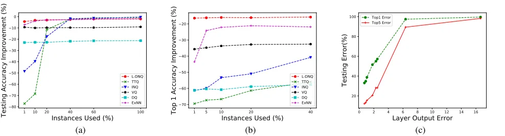
(c)
Figure 2: Fig.(a)/(b): Performance among L-DNQ, ExNN, TTQ, INQ, VQ, DQ using ResNet20/18 in CIFAR10/ImageNet with increasing instances. X-axis presents portion of training data used, Y-axis represents performance improvement after quantization (Higher the better). Fig.(c): Performance under different layer output error. X-axis presents final layer output error, Y-axis represents testing error after quantization (the lower the better).
Network 3-bit 5-bit 7-bit 9-bit Full Precision ResNet18 -16.43/-10.67 -8.61/-4.92 -4.67/-2.40 -2.73/-0.90 69.76/89.02 ResNet34 -29.31/-18.37 -11.22/-6.10 -3.69/-1.88 -2.10/-0.87 73.30/91.42 ResNet50 -19.66/-11.32 -7.55/-4.10 -2.79/-1.24 -1.71/-0.53 76.15/92.87
Table 3: Overall experimental results of L-DNQ in various models using 1% of ImageNet dataset. Column 2-5 represent the quantization improvement (Top1/Top5) under different bits quantization. The last column represents full precision accuracy.
Dataset Network Method kbits TopK Improvement Full Precision (%)
CIFAR10 ResNet20 L-DNQ
− 3 1 -13.66
91.5 L-DNQ 3 1 -4.3
ImageNet AlexNet L-DNQ
− 3 1/5 -56.80/-79.30
58.34/80.80 L-DNQ 3 1/5 -17.78/-14.00
Table 4: Comparison between L-DNQ and L-DNQ−.
For TRN, since it doesn’t release the source code, we com-pare with its reported result using AlexNet. As Table 2 shows, L-DNQ achieves much better performance compared with other methods using 3 bits. In practice, DQ uses more bits in quantization, hence we also compare our model us-ing 9 bits with DQ usus-ing more bits from 8 to 32 in ResNet18 and other baselines with more bits in AlexNet. Clearly, the baseline models retrieve better performances as the number of bits increases, but still hardly achieve comparable per-formances as L-DNQ, which almost approximates the full-precision model with 9 bits.
We also compare L-DNQ, ExNN, TTQ, INQ, VQ and DQ in ResNet20/18 using increasing number of training in-stances on CIFAR-10 and ImageNet. As Fig 2(a) and 2(b) show, L-DNQ maintains high performances even when only a few training instances are used, while training-based meth-ods degrade severely if data is scarce. We conjecture that L-DNQ minimizes the divergence from original network under quantized constraints instead of regenerating a new network given label supervisions, which enables L-DNQ to utilize much less data to preserve the original performance.
Analysis of L-DNQ
Bits’ Effect Towards Performance We conduct experi-ments on various quantization levels on ImageNet using 1% instances. As Table 3 shows, the prediction accuracy in-creases as the number of bits inin-creases. It can be observed that L-DNQ approximately recovers the original accuracy under 9-bit quantization.
Layer Output Error V.S. Performance L-DNQ aims at minimizing the final layer output error between original and quantized networks. It is interesting to explore the relation-ship between layer output error and performance of quan-tized network. We measure the performance of quanquan-tized ResNet18 network on ImageNet dataset under different final output errors. As Fig. 2(c) shows, testing error increases as the final output error increases. Empirically, testing error is positively correlated with final output error. Hence, by mini-mizing the final output error, L-DNQ is capable of attaining good performance.
be considered as a reduction of the proposed L-DNQ. Com-parison results between L-DNQ and L-DNQ−are shown in Table 4: weights update in L-DNQ brings significant perfor-mance gain by narrowing the divergence between quantized network and the unquantized one.
Conclusion
In this paper, we propose a novel layer-wise quantization framework, L-DNQ, and provide a theoretical guarantee on the overall error. We conduct extensive experiments on two benchmark datasets to demonstrate that L-DNQ is able to quantize deep models without big performance drop using only limited training data Therefore, L-DNQ is very effec-tive in the cases where training instances are difficult to at-tain because of data privacy issue and when quantization is deployed in edge devices with limited storage space.
Acknowledgements
This work is supported by NTU Singapore Nanyang Assis-tant Professorship (NAP) grant M4081532.020, Singapore MOE AcRF Tier-1 grant 2016-T1-001-159 and Singapore MOE AcRF Tier-2 grant MOE2016-T2-2-060.
References
Aghasi, A.; Abdi, A.; Nguyen, N.; and Romberg, J. 2017. Net-trim: Convex pruning of deep neural networks with per-formance guarantee. InNIPS. 3180–3189.
Boyd, S.; Parikh, N.; Chu, E.; Peleato, B.; and Eckstein, J. 2011. Distributed optimization and statistical learning via the alternating direction method of multipliers. Found. Trends Mach. Learn.3(1):1–122.
Courbariaux, M.; Bengio, Y.; and David, J. 2015. Bi-naryconnect: Training deep neural networks with binary weights during propagations.CoRRabs/1511.00363. Dong, X.; Chen, S.; and Pan, S. 2017. Learning to prune deep neural networks via layer-wise optimal brain surgeon. InNIPS. 4860–4874.
Gong, Y.; Liu, L.; Yang, M.; and Bourdev, L. 2014. Com-pressing deep convolutional networks using vector quantiza-tion.arXiv preprint arXiv:1412.6115.
Han, S.; Pool, J.; Tran, J.; and Dally, W. 2015. Learning both weights and connections for efficient neural network. InNIPS, 1135–1143.
Hassibi, B., and Stork, D. G. 1993. Second order derivatives for network pruning: Optimal brain surgeon. InNIPS, 164– 171.
He, K.; Zhang, X.; Ren, S.; and Sun, J. 2016. Deep residual learning for image recognition. InCVPR, 770–778. Hou, L., and Kwok, J. T. 2018. Loss-aware weight quanti-zation of deep networks.
Hou, L.; Yao, Q.; and Kwok, J. T. 2016. Loss-aware bina-rization of deep networks.arXiv preprint arXiv:1611.01600. Hubara, I.; Courbariaux, M.; Soudry, D.; El-Yaniv, R.; and Bengio, Y. 2016. Binarized neural networks. InNIPS, 4107– 4115.
Jacob, B.; Kligys, S.; Chen, B.; Zhu, M.; Tang, M.; Howard, A.; Adam, H.; and Kalenichenko, D. 2017. Quantization and training of neural networks for efficient integer-arithmetic-only inference.arXiv preprint arXiv:1712.05877.
Krizhevsky, A.; Sutskever, I.; and Hinton, G. E. 2012. Imagenet classification with deep convolutional neural net-works. InNIPS, 1097–1105.
Kundu, A.; Banerjee, K.; Mellempudi, N.; Mudigere, D.; Das, D.; Kaul, B.; and Dubey, P. 2017. Ternary residual networks. arXiv preprint arXiv:1707.04679.
LeCun, Y.; Denker, J. S.; and Solla, S. A. 1990. Optimal brain damage. InNIPS. 598–605.
Leng, C.; Li, H.; Zhu, S.; and Jin, R. 2017. Extremely low bit neural network: Squeeze the last bit out with admm. In
AAAI.
Li, H.; De, S.; Xu, Z.; Studer, C.; Samet, H.; and Goldstein, T. 2017. Training quantized nets: A deeper understanding. InNIPS, 5811–5821.
Li, F.; Zhang, B.; and Liu, B. 2016. Ternary weight net-works. arXiv preprint arXiv:1605.04711.
Lin, D.; Talathi, S.; and Annapureddy, S. 2016. Fixed point quantization of deep convolutional networks. InICML, 2849–2858.
Lin, X.; Zhao, C.; and Pan, W. 2017. Towards accurate binary convolutional neural network. InNIPS, 344–352. Polino, A.; Pascanu, R.; and Alistarh, D. 2018. Model com-pression via distillation and quantization.
Rastegari, M.; Ordonez, V.; Redmon, J.; and Farhadi, A. 2016. Xnor-net: Imagenet classification using binary con-volutional neural networks. InECCV, 525–542. Springer. Simonyan, K., and Zisserman, A. 2014. Very deep convo-lutional networks for large-scale image recognition. arXiv preprint arXiv:1409.1556.
Takapoui, R.; Moehle, N.; Boyd, S.; and Bemporad, A. 2017. A simple effective heuristic for embedded mixed-integer quadratic programming. International Journal of Control1–11.
Vanhoucke, V.; Senior, A.; and Mao, M. Z. 2011. Improving the speed of neural networks on cpus. InNIPS Workshop on Deep Learning and Unsupervised Feature Learning. Wu, J.; Leng, C.; Wang, Y.; Hu, Q.; and Cheng, J. 2016. Quantized convolutional neural networks for mobile de-vices. InCVPR, 4820–4828.