Random Feature-based Online Multi-kernel Learning
in Environments with Unknown Dynamics
Yanning Shen [email protected]
Tianyi Chen [email protected]
Georgios B. Giannakis [email protected]
Department of Electrical and Computer Engineering, University of Minnesota Minneapolis, MN, 55455, USA
Editor:Karsten Borgwardt
Abstract
Kernel-based methods exhibit well-documented performance in various nonlinear learn-ing tasks. Most of them rely on a preselected kernel, whose prudent choice presumes task-specific prior information. Especially when the latter is not available, multi-kernel learning has gained popularity thanks to its flexibility in choosing kernels from a pre-scribed kernel dictionary. Leveraging the random feature approximation and its recent orthogonality-promoting variant, the present contribution develops a scalable multi-kernel learning scheme (termed Raker) to obtain the sought nonlinear learning function ‘on the fly,’ first for static environments. To further boost performance in dynamic environments, an adaptive multi-kernel learning scheme (termed AdaRaker) is developed. AdaRaker ac-counts not only for data-driven learning of kernel combination, but also for the unknown dynamics. Performance is analyzed in terms of both static and dynamic regrets. AdaRaker is uniquely capable of tracking nonlinear learning functions in environments with unknown dynamics, and with with analytic performance guarantees. Tests with synthetic and real datasets are carried out to showcase the effectiveness of the novel algorithms.1
Keywords: Online learning, reproducing kernel Hilbert space, multi-kernel learning, random features, dynamic and adversarial environments.
1. Introduction
Function approximation emerges in various learning tasks such as regression, classification, clustering, dimensionality reduction, as well as reinforcement learning (Sch¨olkopf and Smola, 2002; Shawe-Taylor and Cristianini, 2004; Dai et al., 2017). Among them, the emphasis here is placed on supervised functional learning tasks: given samples {(x1, y1), . . . ,(xT, yT)}Tt=1 with xt ∈ Rd and yt ∈ R, the goal is to find a function f(·) such that the discrepancy between each pair ofytandf(xt) is minimized. Typically, such discrepancy is measured by
a cost functionC(f(xt), yt), which requires to findf(·) minimizingPTt=1C(f(xt), yt). While
this goal is too ambitious to achieve in general, the problem becomes tractable when f(·) is assumed to belong to a reproducing kernel Hilbert space (RKHS) induced by a kernel
(Sch¨olkopf and Smola, 2002). Comparable to deep neural networks, functions defined in
1. Preliminary results in this paper were presented in part at the 2018 International Conference on Artificial Intelligence and Statistics (Shen et al., 2018).
c
RKHS can model highly nonlinear relationship, and thus kernel-based methods have well-documented merits for principled function approximation. Despite their popularity, most kernel methods rely on a single pre-selected kernel. Yet, multi-kernel learning (MKL) is more powerful, thanks to its data-driven kernel selection from a given dictionary; see e.g., (Shawe-Taylor and Cristianini, 2004; Rakotomamonjy et al., 2008; Cortes et al., 2009; G¨onen and Alpaydın, 2011), and (Bazerque and Giannakis, 2013).
In addition to the attractive representation power that can be afforded by kernel meth-ods, several learning tasks are also expected to be performed in an online fashion. Such a need naturally arises when the data arrive sequentially, such as those in online spam detec-tion (Ma et al., 2009), and time series predicdetec-tion (Richard et al., 2009); or, when the sheer volume of data makes it impossible to carry out data analytics in batch form (Kivinen et al., 2004). This motivates well online kernel-based learning methods that inherit the merits of their batch counterparts, while at the same time allowing efficient online implementation. Taking a step further, the optimal function may itself change over time in environments withunknown dynamics. This is the case when the function of interest e.g., represents the state in brain graphs, or, captures the temporal processes propagating over time-varying networks. Especially when variations are due to adversarial interventions, the underlying dynamics are unknown. Online kernel-based learning in such environments remains a largely uncharted territory (Kivinen et al., 2004; Hoi et al., 2013).
In accordance with these needs and desiderata, thegoal of this paper is an algorithmic pursuit of scalable online MKL in environments with unknown dynamics, along with their associated performance guarantees. Major challenges come from two sources: i) the well-known “curse” of dimensionality in kernel-based learning; and, ii) the defiance of tracking unknown time-varying functions without future information. Regarding i), the representer theorem renders the size of kernel matrices to grow quadratically with the number of data
(Wahba, 1990), thus the computational complexity to find even a single kernel-based
pre-dictor is cubic. Furthermore, storage of past data causes memory overflow in large-scale learning tasks such as those emerging in e.g., topology identification of social and brain networks (Shen et al., 2016, 2017; Shen and Giannakis, 2018), which makes kernel-based methods less scalable relative to their linear counterparts. For ii), most online learning set-tings presume time invariance or slow dynamics, where an algorithm achieving sub-linear regret incurs on average “no-regret” relative to thebest static benchmark. Clearly,
design-ing online schemes that are comparable to the best dynamic solution is appealing though
formidably challenging without knowledge of the dynamics (Kivinen et al., 2004).
1.1. Related works
To put our work in context, we review prior art from the following two aspects.
con-siderably reduced through an orthogonality promoting RF modification (Yu et al., 2016). These approaches assume that the kernel is known, a choice crucially dependent on domain knowledge. Enabling kernel selection, several MKL-based approaches have emerged, see e.g., (Lanckriet et al., 2004; Rakotomamonjy et al., 2008; Bach, 2008; Cortes et al., 2009;
G¨onen and Alpaydın, 2011), and their performance gain has been documented relative to
their single kernel counterparts. However, the aforementioned methods are designed for batch settings, and are either intractable or become less efficient in online setups. When the sought functions vary over time and especially when the dynamics are unknown (as in adversarial settings), batch schemes fall short in tracking the optimal function estimators.
Online (multi-)kernel learning. Tailored for streaming large-scale datasets, online kernel-based learning methods have gained due popularity. To deal with the growing
com-plexity of online kernel learning, successful attempts have been made to design budgeted
kernel learning algorithms, including techniques such as support vector removal (Kivinen et al., 2004; Dekel et al., 2008), and support vector merging (Wang et al., 2012). Maintain-ing an affordable budget, online multi-kernel learnMaintain-ing (OMKL) methods have been reported for online classification (Jin et al., 2010; Hoi et al., 2013; Sahoo et al., 2016), and regression (Sahoo et al., 2014; Lu et al., 2018). Devoid of the need for budget maintenance, online kernel-based learning algorithms based on RF approximation (Rahimi and Recht, 2007) have been developed in (Lu et al., 2016; Bouboulis et al., 2018; Ding et al., 2017), but only with a single pre-selected kernel. More importantly, existing kernel-based learning
ap-proaches implicitly presume astatic environment, where the benchmark is provided through
the best static function (a.k.a. static regret) (Shalev-Shwartz, 2011). However, static regret is not a comprehensive metric for dynamic settings, where the optimal kernel also varies over time and the dynamics are generally unknown as with adversarial settings.
1.2. Our contributions
The present paper develops an adaptive online MKL algorithm, capable of learning a nonlin-ear function from sequentially arriving data samples. Relative to prior art, our contributions can be summarized as follows.
c1)For the first time, RFs are employed for scalable online MKL tackled by a weighted combination of advices from an ensemble of experts - an innovative cross-fertilization of
online learning to MKL. Performance of the resultant algorithm (abbreviated asRaker) is
benchmarked by the best time-invariant function approximant via static regret analysis.
c2) A novel adaptive approach (termed AdaRaker) is introduced for scalable online
MKL in environments with unknown dynamics. AdaRaker is a hierarchical ensemble learner with scalable RF-based modules that provably yields sub-linear dynamic regret, so long as the accumulated variation grows sub-linearly with time.
c3)The novel algorithms are compared with competing alternatives for online nonlinear
regression on both synthetic and real datasets. The tests corroborate that Raker and
AdaRaker exhibit attractive performance in both accuracy and scalability.
Notation. Bold uppercase (lowercase) letters will denote matrices (column vectors), while (·)> stands for vector and matrix transposition, andkxkdenotes the`2-norm of a vectorx. Inequalities for vectors x > 0, and the projection operator [a]+ := max{a,0} are defined entrywise. Symbol † represents the Hermitian operator, while the indicator function 1{A}
takes value 1 when the eventAhappens, and 0 otherwise. Edenotes the expectation, while
h·,·i andh·,·iH the vector inner product in Euclidian and Hilbert space respectively.
2. Preliminaries and Problem Statement
This section reviews briefly basics of kernel-based learning, to introduce notation and the needed background for our novel online MKL schemes.
Given samples {(x1, y1), . . . ,(xT, yT)}tT=1 with xt ∈ Rd and yt ∈ R, the function ap-proximation task is to find a function f(·) such that yt =f(xt) +et, where et denotes an
error term representing noise or un-modeled dynamics. It is supposed thatf(·) belongs to a reproducing kernel Hilbert space (RKHS), namelyH:={f|f(x) =P∞
t=1αtκ(x,xt)}, where
κ(x,xt) :Rd×Rd→ Ris a symmetric positive semidefinite basis (so-termed kernel)
func-tion, which measures the similarity between x and xt. Among the choices of κ specifying
different bases, a popular one is the Gaussian given byκ(x,xt) := exp[−kx−xtk2/(2σ2)]. A
kernel is reproducing if it satisfies hκ(x,xt), κ(x,xt0)iH=κ(xt,xt0), which in turn induces the RKHS norm kfk2
H:= P
t
P
t0αtαt0κ(xt,xt0). Consider the optimization problem
min
f∈H 1
T
T
X
t=1
C(f(xt), yt) +λΩ kfk2H
(1)
where depending on the application, the cost functionC(·,·) can be selected to be, e.g., the least-squares (LS), the logistic or the hinge loss; Ω(·) is an increasing function; and,λ >0 is a regularization parameter that controls overfitting. According to the representer theorem, the optimal solution of (1) admits the finite-dimensional form, given by (Wahba, 1990)
ˆ
f(x) =
T
X
t=1
αtκ(x,xt) :=α>k(x) (2)
where α := [α1, . . . , αT]>∈ RT collects the combination coefficients, and the T ×1 ker-nel vector is k(x) := [κ(x,x1), . . . , κ(x,xT)]>. Substituting (2) into the RKHS norm, we
find kfk2 H :=
P
t
P
t0αtαt0κ(xt,xt0) = α>Kα, where the T ×T kernel matrix K has en-tries [K]t,t0 := κ(xt,xt0); thus, the functional problem (1) boils down to a T-dimensional optimization overα, namely
min α∈RT
1
T
T
X
t=1
C(α>k(xt), yt) +λΩ
α>Kα
(3)
where k>(xt) is the tth row of the matrix K. While a scalar yt is used here for brevity,
coverage extends readily to vectors{yt}.
(3) grows with timeT (or, the number of samples in the batch form), making it less scalable in online implementation. In the ensuing section, an online MKL method will be proposed to select κ as a superposition of multiple kernels, when the data become available online.
3. Online MKL in static environments
In this section, we develop an online learning approach that builds on the notion of random features (Rahimi and Recht, 2007; Yu et al., 2016), and leverages in a unique way multi-kernel approximation – two tools justifying our acronymRaker used henceforth.
3.1. RF-based single kernel learning
To cope with the curse of dimensionality in optimizing (3), we will reformulate the functional optimization problem (1) as a parametric one with the dimension of optimization variables not growing with time. In this way, powerful toolboxes from convex optimization and online learning in vector spaces can be leveraged. We achieve this goal by judiciously using RFs. Although generalizations will follow, this subsection is devoted to RF-based single kernel learning, where basics of kernels, RFs, and online learning will be revisited.
As in (Rahimi and Recht, 2007), we will approximate κ in (2) using shift-invariant
kernels that satisfyκ(xt,xt0) =κ(xt−xt0). Forκ(xt−xt0) absolutely integrable, its Fourier transform πκ(v) exists and represents the power spectral density, which upon normalizing
to ensureκ(0) = 1, can also be viewed as a probability density function (pdf); hence,
κ(xt−xt0) = Z
πκ(v)ejv
>(x
t−xt0)dv:=Evejv>(xt−xt0) (4)
where the last equality is just the definition of the expected value. Drawing a sufficient number of D independent and identically distributed (i.i.d.) samples {vi}D
i=1 from πκ(v),
the ensemble mean in (4) can be approximated by the sample average
ˆ
κc(xt,xt0) := 1 D
D
X
i=1
ejv>i (xt−xt0):=ζ†
V(xt)ζV(xt0) (5)
whereV:= [v1, . . . ,vD]> ∈RD×d, symbol†represents the Hermitian (conjugate-transpose)
operator, andζV(x) the complex RF vector
ζV(x) := 1 √
D h
ejv>1x, . . . , ejv>Dx
i>
. (6)
Taking expected values on both sides of (5) and using (4) yieldsEv[ˆκc(xt,xt0)] =κ(xt,xt0), which means ˆκc is unbiased. Likewise, ˆκc can be shown consistent since Var[ˆκc(xt,xt0)]∝
D−1 vanishes as D → ∞. Finding πκ(v) requires d-dimensional Fourier transform of κ,
generally through numerical integration. For a number of popular kernels however, πκ(v)
is available in closed form. Taking the Gaussian kernel as an example, whereκG(xt,xt0) = exp kxt−xt0k2
2/(2σ2)
, has Fourier transform corresponding to the pdfπG(v) =N(0, σ−2I).
Instead of thecomplex RFs{ζV(xt)}in (6) forming the linear kernel estimator ˆκcin (5),
of κ. Defining the real RF vector zV(x) := [<>{ζV(xt)},=>{ζV(xt)}]>, this real kernel
estimator becomes (cf. (5))
ˆ
κ(xt,xt0) =zV>(xt)zV(xt0) (7)
where the 2D×1real RF vector can be written as
zV(x) = 1 √
D h
sin(v>1x), . . . ,sin(v>Dx),cos(v>1x), . . . ,cos(v>Dx) i>
. (8)
Hence, the nonlinear function that is optimal in the sense of (1) can be approximated by a linear one in the new 2D-dimensional RF space, namely (cf. (2) and (7))
ˆ
fRF(x) =
T
X
t=1
αtz>V(xt)zV(x) :=θ>zV(x) (9)
whereθ> :=PT
τ=1ατz>V(xτ) is the new weight vector of size 2Dwhose dimension does not
increase with number of data samples T.
While the solution ˆf in (2) is the superposition of nonlinear functionsκ, its RF approx-imant ˆfRFin (9) is a linear function of zV(x). As a result, the loss becomes
Lt f(xt)
:=C(f(xt), yt) +λΩ kfk2H
=C θ>zV(xt), yt
+λΩ kθk2
(10)
wherekθk2 :=P
t
P
t0αtαt0z>
V(xt)zV(xt0) :=kfk2H; and the online learning task is min
θ∈R2D
T
X
t=1
Lθ>zV(xt), yt
, withL θ>zV(xt), yt
:=C θ>zV(xt), yt
+λΩ kθk2 . (11)
Compared with the functional optimization in (1), the reformulated problem (11) is para-metric, and more importantly it involves only optimization variables of fixed size 2D. We can thus solve (11) using the online gradient descent iteration, e.g., (Hazan, 2016). Acquir-ingxt per slot t, its RFzV(xt) is formed as in (8), andθt+1 is updated online as
θt+1 =θt−ηt∇L(θ>t zV(xt), yt) (12)
where{ηt}is the sequence of stepsizes that can tune learning rates, and ∇L(θt>zV(xt), yt)
the gradient atθ=θt. Iteration (12) providesa functional updatesince ˆftRF(x) =θ>tzV(x), but the upshot of involving RFs is that this approximant is in the span of{zV(x),∀x∈ X }. Since E[ˆκ] = κ, we find readily that E[ ˆfRF] = ˆf; in words, unbiasedness of the kernel approximation ensures that the RF-based function approximant is also unbiased.
Variance-reduced RF. Besides unbiasedness, performance of the RF approximation is
also influenced by the variance of RFs. Note that the variance of ˆκ in (7) is of order
O(D−1), but its scale can be reduced if V is formed to have orthogonal rows (Yu et al., 2016). Specifically for a Gaussian kernel with bandwidthσ2, recall that V=σ−1Gin (8),
with D = d, one starts with Q-R factorization of V =QR, and uses the d×d factor Q along with a diagonal matrixΛ, to form (Yu et al., 2016)
VORF=σ−1ΛQ (13)
where the diagonal entries of Λ are drawn i.i.d. from the χ distribution with ddegrees of freedom, to ensure unbiasedness of the kernel approximant. ForD > d, one selects D=νd
with ν > 1 integer, and generates independently ν matrices each of size d×d as in (13).
The finalVORFis formed by concatenating thesed×dsub-matrices. The upshot of ORF is
that (Yu et al., 2016) Var(ˆκORF(xt,xt0))≤Var(ˆκ(xt,xt0)). As we have also confirmed via simulated tests, ORF-based function approximation can attain a prescribed accuracy with considerably less ORFs than what required by its RF-based counterpart.
The RF-based online single kernel learning scheme in this section presumes that κ is
known a priori. Since this is not generally possible, it is prudent to adaptively select kernels by superimposing multiple kernel functions from a prescribed dictionary. This superposition will play a key role in the RF-based online MKL approach presented next.
3.2. Raker for online MKL
Specifying the kernel that “shapes”His a critical choice for single kernel learning, since dif-ferent kernels yield function estimates of variable accuracy. To deal with this, combinations of kernels from a prescribed and sufficiently rich dictionary{κp}Pp=1 can be employed in (1). Each combination belongs to the convex hull ¯K:={¯κ=PP
p=1α¯pκp,α¯p ≥0,PPp=1α¯p = 1},
and is itself a kernel (Sch¨olkopf and Smola, 2002). With ¯H denoting the RKHS induced
by ¯κ ∈ K, one then solves (1) with¯ H replaced by ¯H := H1L· · ·LHP, where {Hp}Pp=1 represent the RKHSs corresponding to{κp}Pp=1 (Micchelli and Pontil, 2005).
The candidate function ¯f ∈H¯ is expressible in a separable form as ¯f(x) :=PP
p=1f¯p(x), where ¯fp(x) belongs to Hp, for p ∈ P := {1, . . . , P}. To add flexibility per kernel in our
ensuing online MKL scheme, we let wlog{f¯p =wpfp}Pp=1, and seek functions of the form
f(x) :=
P
X
p=1 ¯
wpfp(x)∈H¯ (14)
wheref := ¯f /PP
p=1wp, and the normalized weights{w¯p :=wp/
PP
p=1wp}Pp=1 satisfy ¯wp≥
0, andPP
p=1w¯p = 1. Plugging (14) into (1), MKL solves the nonconvex problem
min {w¯p},{fp}
1
T
T
X
t=1 C
P
X
p=1 ¯
wpfp(xt), yt
+λΩ
P
X
p=1 ¯
wpfp
2
¯ H
(15a)
s.to
P
X
p=1 ¯
wp= 1, w¯p ≥0, p∈ P (15b)
fp ∈ Hp, p∈ P. (15c)
If Ω is convex over f, then (15a) is biconvex, meaning it is convex wrt {fp} ({w¯p}) when
alternating minimization that is known not to scale well withP andT (Micchelli and Pontil, 2005; Cortes et al., 2009; G¨onen and Alpaydın, 2011).
To deal with scalability, our novel approach will leverage for the first time (O)RFs in a uniquely principled MKL formulation to end up with an efficient online learning approach. To this end, we will minimize a cost that upper bounds that in (15a), namely
min {w¯p},{fp}
1
T
T
X
t=1 P
X
p=1 ¯
wpC(fp(xt), yt) +λ P
X
p=1 ¯
wpΩ
kfpk2Hp
s.to (15b) and (15c) (16)
where Jensen’s inequality confirms that under (15b) the cost in (16) upper bounds that of (15a). A key advantage of (16) is that its objective is separable across kernel ‘atoms.’
We will exploit this separability jointly with the RF-based function approximation per kernel, to formulate our scalable online MKL task as
min {w¯p},{fˆpRF}
T
X
t=1 P
X
p=1 ¯
wpLt
ˆ
fpRF(xt)
s.to (15b) and ˆfpRF∈nfˆp(x) =θ>zVp(x)
o
(17)
where we interchangeably useLt( ˆf(xt)) as defined in (10) and L θ>zV(xt), yt
as in (11). We will efficiently solve (17) ‘on-the-fly’ using our Raker algorithm, and what more, we will provide analytical performance guarantees. Our iterative solution will update separately each ˆfpRF as in Section 3.1 using the scalable (O)RF-based function approximation scheme. Given xt, an RF vectorzp(xt) will be generated per p from pdf πκp(v) (cf. (8)), where we
let zp(xt) :=zVp(xt) for notational brevity. Hence, for eachp and slott, we have
ˆ
fp,tRF(xt) =θ>p,tzp(xt) (18)
and as in (12),θp,t is updated via
θp,t+1 =θp,t−η∇L(θp,t>zp(xt), yt). (19)
As far as solving for ¯wp,t, since it resides on a probability simplex (15b), our idea is
to employ a multiplicative update (a.k.a. exponentiated gradient descent), e.g., (Hazan, 2016). Specifically, the un-normalized weights are found first as
wp,t+1 = arg min wp
ηLtfˆp,tRF(xt)
(wp−wp,t) +DKL(wpkwp,t) (20)
whereDKL(wpkwp,t) :=wplog(wp/wp,t) is the KL-divergence. It can be readily verified that
(20) admits the following closed-form update
wp,t+1 =wp,texp
−ηLt
ˆ
fp,tRF(xt)
(21)
where η ∈ (0,1) is a chosen constant that controls the adaptation rate of {wp,t}. Having
found{wp,t}as in (21), the normalized weights in (14) are obtained as ¯wp,t:=wp,t/
PP p=1wp,t.
Update (21) is intuitively pleasing because when ˆfRF
p,t contributes a larger loss relative to
Algorithm 1 Raker for online MKL in static environments
1: Input:Kernels κp, p= 1, . . . , P, step size η >0, and number of random features D. 2: Initialization:θ1 =0.
3: fort= 1,2, . . . , T do
4: Receive a streaming datum xt.
5: Construct zp(xt) via (8) using κp forp= 1, . . . , P.
6: Predict ˆftRF(xt) :=PPp=1w¯p,tfˆp,tRF(xt) with ˆfp,tRF(xt) in (18). 7: Observe loss functionLt, incur Lt( ˆftRF(xt)).
8: for p= 1, . . . , P do
9: Obtain lossL(θ>p,tzp(xt), yt) or Lt( ˆfp,tRF(xt)).
10: Updateθp,t+1 via (19).
11: Updatewp,t+1 via (21).
12: end for 13: end for
weights in the next time slot. In other words, a more accurate RF-based approximant tends to play more important role in predicting the upcoming data.
Remark 1. The update (21) resembles the online learning paradigm, a.k.a. online predic-tion with (weighted) expert advices (Vovk, 1995; Cesa-Bianchi and Lugosi, 2006). Building on but going beyond OMKL in (Sahoo et al., 2014), the idea here is to view MKL with
RF-based function approximants as a weighted combination of advices from an ensemble
of P function approximants (experts). Besides permeating benefits from online learning to
MKL, what is distinct here relative to (Vovk, 1995; Cesa-Bianchi and Lugosi, 2006) is that each function approximant also performs online learning for self improvement (cf. (19)).
In summary, our Raker for static (or slow-varying) dynamics is listed as Algorithm 1.
Memory requirement and computational complexity. At the t-th iteration, our
Raker in Algorithm 1 needs to store a real 2D RF vector, and its corresponding weight
vector per κp. Hence, the memory required is of order O(dDP). Regarding computational
overhead, the per-iteration complexity (e.g., calculating inner products) is again of order
O(dDP). Compared with the complexity ofO(tdP) for OMKL by (Sahoo et al., 2014), or,
O(t3P) when matrix inversion required for the batch MKL, e.g., (Bazerque and Giannakis,
2013), the Raker is clearly more scalable, as t grows. Even when OMKL is confined to a
budget ofB past samples, the corresponding complexity ofO(dBP) is comparable to that
of Raker. This speaks for Raker’s merits, whose performance guarantees will be proved analytically, and also demonstrated by numerical tests to outperform budgeted schemes.
Application examples: Online MKL regression and classification. To appreciate the usefulness of RF-based online MKL, consider first nonlinear regression, where given samples {xt ∈ Rd, yt ∈ R}Tt=1, the goal is to find a nonlinear function f ∈ H, such that
yt=f(xt) +et. The criterion is to minimize the regularized prediction error ofyt, typically
using the LS loss L(f(xt), yt) := [yt−f(xt)]2+λkfk2H, whose gradient is (cf. (19)) ∇Lθ>p,tzp(xt), yt
It is clear that the per iteration complexity of Raker is only related to the dimension of zp(xt), and does not increase over time.
For nonlinear classification, consider kernel-based perceptron and kernel-based logistic regression, which aim at learning a nonlinear classifier that best approximates eitheryt or
the pdf of yt conditioned on xt. With binary labels {±1}, the perceptron solves (1) with
L(f(xt), yt) = max(0,1−ytf(xt)) +λkfk2H, which equals zero if yt =f(xt), otherwise it
equals 1. Raker’s gradient in this case is (cf. (19))
∇Lθ>p,tzp(xt), yt
=−2ytC(θ>p,tzp(xt), yt)zp(xt) + 2λθp,t. (23)
Accordingly, givenxt, logistic regression postulates that Pr(yt= 1|xt) = 1/(1 + exp(f(xt))).
Here the gradient of Raker takes the form (cf. (19))
∇Lθ>p,tzp(xt), yt
= 2ytexp(ytθ >
p,tzp(xt))
1 + exp(ytθ>p,tzp(xt))
zp(xt) + 2λθp,t. (24)
To compare alternatives on equal footing, the numerical tests in Section 5 will deal with kernel-based regression and classification.
3.3. Static regret analysis of Raker
To analyze the performance of Raker, we assume that the following conditions are satisfied. (as1)Per slot t, the loss function L(θ>zV(xt), yt) in (11) is convex w.r.t. θ.
(as2) For θ belonging to a bounded set Θ with kθk ≤ Cθ, the loss is bounded; that is,
L(θ>zV(xt), yt)∈[−1,1], and has bounded gradient, meaning, k∇L(θ>zV(xt), yt)k ≤L.
(as3)Kernels {κp}Pp=1 are shift-invariant, standardized, and bounded, that is, κp(xi,xj)≤
1,∀xi,xj; and w.l.o.g. they also have bounded entries, meaning kxk ≤1.
Convexity of the loss under (as1) is satisfied by the popular loss functions including the square loss and the hinge loss. As far as (as2), it ensures that the losses, and their
gradients are bounded, meaning they are L-Lipschitz continuous. While boundedness of
the losses commonly holds sincekθkis bounded, Lipschitz continuity is also not restrictive. Considering kernel-based regression as an example, the gradient is (θ>zV(xt)−yt)zV(xt) +
λθ. Since the loss is bounded, e.g., kθ>zV(xt)−ytk ≤ 1, and the RF vector in (8) can
be bounded as kzV(xt)k ≤ 1, the constant is L := 1 +λCθ using the Cauchy-Schwartz
inequality. Kernels satisfying conditions in (as3) include Gaussian, Laplacian, and Cauchy (Rahimi and Recht, 2007). In general, (as1)-(as3) are standard in online convex optimization (OCO) (Shalev-Shwartz, 2011; Hazan, 2016), and in kernel-based learning (Micchelli and Pontil, 2005; Rahimi and Recht, 2007; Lu et al., 2016).
With regard to the performance of an online algorithm, static regret is commonly adopted as a metric by most OCO schemes to measure the difference between the ag-gregate loss of an OCO algorithm, and that of the best fixed function approximant in hindsight, e.g., (Shalev-Shwartz, 2011; Hazan, 2016). Specifically, for a generic sequence {fˆt}generated by an RF-based kernel learning algorithm A, its static regret is
RegsA(T) :=
T
X
t=1
Lt( ˆft(xt))− T
X
t=1
where ˆft will henceforth represent ˆftRF without the superscript for notational brevity; and,
f∗(·) is obtained as the batch solution
f∗(·)∈arg min {f∗
p, p∈P}
T
X
t=1
Lt(fp∗(xt)) with fp∗(·)∈arg min f∈Fp
T
X
t=1
Lt(f(xt)) (26)
with Fp := Hp, and Hp representing the RKHS induced by κp. Using (25) and (26), we
first establish the static regret of our Raker approach in the following lemma.
Lemma 1 Under (as1), (as2), and withfˆp∗as in (26)withFp :={fˆp|fˆp(x) =θ>zp(x),∀θ∈
R2D}, the sequences {fˆp,t} and{w¯p,t} generated by Raker satisfy the following bound T
X
t=1 Lt
P
X
p=1 ¯
wp,tfˆp,t(xt)
−
T
X
t=1
Ltfˆp∗(xt)
≤ lnP
η +
kθ∗pk2
2η +
ηL2T
2 +ηT (27)
where θ∗p is associated with the best RF function approximant fˆp∗(x) = θ∗p>zp(x).
Proof: See Appendix A.
Besides Raker’s static regret bound, the next theorem compares the Raker loss relative to that of the best functional estimator in the original RKHS.
Theorem 1 Under (as1)-(as3) and withfp∗ in (26) belonging to the RKHSHp, for a fixed
>0, the following bound holds with probability at least1−28 σp
2
exp −4dD+82
T
X
t=1 Lt
P
X
p=1 ¯
wp,tfˆp,t(xt)
− min
p∈{1,...,P}
T
X
t=1
Lt fp∗(xt)
≤lnP
η +
(1 +)C2
2η +
ηL2T
2 +ηT+LT C (28)
where C is a constant, whileσ2p :=EπVκp[kvk2]is the second-order moment of the RF vector
norm. Setting η==O(1/√T) in (28), the static regret in (25) leads to
RegsRaker(T) =O(√T). (29)
Proof: See Appendix B.
Observe that the probability of (28) to hold grows as D increases, and one can always
find a D to ensure a positive probability for a given . Bearing this in mind, we will
AdaRaker
…
…
P kernels P kernels
…
Raker
…
…
Adaptivity
…
…
Figure 1: Hierarchical AdaRaker structure. Experienced experts in the middle layer present a Raker instance, where the size of expert cartoons is proportional to the interval length.
4. Online MKL in Environments with Unknown Dynamics
Our Raker in Section 3 combines an ensemble of kernel learners ‘on the fly,’ and performs on average as the “best” fixed function, thus fulfilling the learning objective in environ-ments with zero (or slow) dynamics. To broaden its scope to environenviron-ments with unknown
dynamics, this section introduces anadaptive Raker approach (termedAdaRaker).
4.1. AdaRaker with hierarchical ensembles
As with any online learning algorithm, the choice of η in (19) and (21) affects the
perfor-mance critically. Especially in environments with unknown dynamics, a large η improves
the tracking ability of fast-varying functions, while a smaller one allows improved estima-tion of slow-varying parameters {θt, wp,t}. The optimal choice of ηt clearly depends on
the variability of the optimal function estimator (Kivinen et al., 2004; Besbes et al., 2015). Selecting{ηt}however, is formidably challenging if the environment dynamics are unknown.
Toward addressing this challenge, our idea here is to hedge between multiple Raker learners with different learning rates. Specifically, we view each Raker instance in Algorithm 1 as a black box algorithm AI, where the subscript I represents the algorithm running on interval I := [I,I¯] starting from slot I to slot ¯I. Let a pre-selected set I collect all these intervals, the design of which will be specified later. At the beginning of each interval
I ∈ I, a new instance of the online Raker algorithm AI is initialized with an interval-specific learning rateη(I):= min{1/2, η0/
p
|I|}with constant η0>0. Allowing for overlap
Algorithm 2 AdaRaker for online MKL in dynamic environments
1: Initialization: learner weights {h(1I)}, and their learning rates {η(I)}. 2: fort= 1,2, . . . , T do
3: Obtain ˆft(I)(xt) from each Raker instance AI,I ∈ I(t). 4: Predict ˆft(xt) via a weighted combination (33).
5: Observe loss functionLt, and incur Lt( ˆft(xt)). 6: for I ∈ I(t)do
7: Incur lossLt( ˆft(I)(xt)).
8: Update ˆft(I) via Raker in Algorithm 1. 9: Update weightsh(t+1I) via (31).
10: end for 11: end for
collecting all active intervals at the current slott in the set
I(t) :={I ∈ I |t∈[I,I¯]}, ∀t∈ T. (30)
For each Raker instance AI with I ∈ I(t), let ˆft(I)(·) denote its output at time t that
combines multiple kernel-based function estimators, and Lt( ˆft(I)(xt)) represent the
associ-ated instantaneous loss. The output of the ensemble learner A at time t is the weighted
combination of outputs from all learners, namely {fˆt(I),∀I ∈ I(t)}. Withh(tI)denoting the weight of the Raker instance AI, we will update it online via
h(tI+1) =
0, ift /∈I
η(I), ift=I
h(tI)exp −η(I)rt(I), else
(31)
whereI is the first time slot of interval I, and the loss of AI relative to the overall loss is
r(tI)=Lt( ˆft(xt))− Lt( ˆft(I)(xt)), ∀I ∈ I(t). (32)
Intuitively thinking, one would wish to decrease (increase) the weights of those instances with small (large) losses in future rounds. Using update (31), and defining the normalized weight as ¯h(tI):=h(tI)/P
J∈I(t)h (J)
t , the overall output is given by
ˆ
ft(x) :=
X
I∈I ¯
h(tI)fˆt(I)(x) with fˆt(I)(x) :=X
p∈P ¯
w(p,tI)fˆp,t(I)(x) (33)
where{w¯p,t(I)}are the kernel combination weights generated by RakerAI (cf. (21)). The AdaRaker scheme is summarized in Algorithm 2, and depicted in Figure 1.
Time
1 2 4
…...
7
In
ter
v
a
l
len
gth
…...
…...
…...
…...
Figure 2: AdaRaker as an ensemble of Rakers with different learning rates: Each light/dark black interval initiates a Raker learner. At slot 7, colored experts are active, and gray ones are inactive.
design is well motivated because with long intervals, the Raker loss per interval is relatively low in slow-varying settings, but higher as the dynamics become more pronounced. On the other hand, a short interval can hedge against a possibly rapid change, but its performance on each interval could suffer if the objective stays nearly static. Bearing these tradeoffs in mind, we present next a simple yet efficient interval partitioning scheme.
Illustration of interval sets: Consider partitioning the entire horizon into intervals of length 20,21,22, . . .. Intervals of length 2j with a given j ∈ N are consecutively assigned without overlap starting from t= 2j. In the non-overlapping case, define a set of intervals
Ij = [Ij,I¯j] such that each interval’s length is |Ij| = ¯Ij −Ij + 1 = 2j, j ∈ N. For this
selection of intervals, each time slot tis covered by a set of at mostdlog2te intervals, which forms the active set of intervals I(t) at time t. See the diagram in Fig. 2.
4.2. Dynamic regret analysis of AdaRaker
The static regret in Theorem 1 is with respect to a time-invariant optimal function estima-tor benchmark. In dynamic environments however, this optimal function benchmark may change over time - what justifies this subsection’s performance analysis of AdaRaker.
Our analysis will rely on the dynamic regret that is related to tracking regret, and has been introduced in (Besbes et al., 2015; Jadbabaie et al., 2015) to quantify the performance of online algorithms. The dynamic regret is defined as (cf. (25))
RegdA(T) :=
T
X
t=1
Lt( ˆft(xt))− T
X
t=1
Lt(ft∗(xt)) (34)
where the benchmark is the aggregate loss incurred by a sequence of the best dynamic functions{ft∗} from F formed by the union of function spaces Hp induced by {κp}, given
by
ft∗(·)∈arg min {f∗
p,t, p∈P}
Lt(fp∗(xt)) with fp,t∗ (·)∈arg min f∈Hp
Comparing (26) with (35) we deduce that the dynamic regret is always larger than the static regret in (25). Thus, a sub-linear dynamic regret implies a sub-linear static regret, but not vice versa. Given{Lt}, AdaRaker generates functions{fˆt}to minimize the dynamic regret.
To assess the AdaRaker performance, we will start with an intermediate result on the
static regret associated with any sub-intervalI ⊆ T.
Lemma 2 Under (as1)-(as3), the static regret on any interval I ⊆ T is given by
RegsA(|I|) := X
t∈I
Lt( ˆft(xt))−
X
t∈I
Lt(fI∗(xt)) (36)
where |I|denotes the length of intervalI, and the best time-invariant function approximant isfI∗ ∈arg minf∈S
p∈PHp
P
t∈ILt(f(xt)), with Hp denoting the RKHS induced byκp. Then
for any interval I ⊆ T and fixed positive constantsC0, C1, the following bound holds RegsAdaRaker(|I|)≤C0
p
|I|+C1lnT
p
|I|, w.h.p. (37)
Proof: See Appendix C.
Lemma 2 establishes that by combining Raker learners with different learning rates,
AdaRaker can achieve sub-linear static regret over any interval I with arbitrary interval
length. This also holds for intervals overlapping with multiple intervals; see e.g., the red interval in Fig. 2. Clearly, the best fixed solution in (36) is interval specific, which can vary over different intervals. This is qualitatively why the function approximants generated by
AdaRaker can cope with a time-varying benchmark. Such an intuition will in fact become
quantitative in the next theorem, which establishes the dynamic regret for AdaRaker.
Theorem 2 Suppose (as1)-(as3) are satisfied, and define the accumulated variation of on-line loss functions as
V({Lt}Tt=1) := T
X
t=1 max
f∈F
Lt+1(f(xt+1))−Lt(f(xt))
(38)
where F :=S
p∈PHp. Then AdaRaker can afford a dynamic regret in (34) bounded by
RegdAdaRaker(T)≤(2 +C0+C1lnT)T
2 3V
1 3({Lt}T
t=1) = ˜OT23V
1 3({Lt}T
t=1)
, w.h.p. (39)
where O˜ neglects the lower-order terms with a polynomiallogT rate.
Proof: See Appendix D.
Intermittent switches: WithLt6=Lt+1 defining a switch, consider that the number of switches is sub-linear overT; that is,PT
t=11(Lt6=Lt+1) =Tγ,∀γ ∈[0,1). Then it follows thatV({Lt}T
t=1) =O(Tγ), since the one-slot variation of the loss functions is bounded. Other setups with sub-linear accumulated variation emerge, e.g., when the per-slot vari-ation decreases asV(Lt) =O(tγ−1),∀γ ∈[0,1). Besides dynamic losses, sub-linear dynamic
regrets can be also effected by confining the variability of optimal function estimators.
Theorem 3 Suppose the conditions of Theorem 2 hold, and define the regret relative to an m-switching dynamic benchmark as RegmA(T) :=
PT
t=1Lt( ˆft(xt))−
PT
t=1Lt( ˇf ∗
t(xt)), where
{fˇt∗} is any trajectory from
n ˇ
ft∗ Tt=1∈S
p∈PHp
PT
t=11( ˇf ∗
t 6= ˇft∗−1)≤m
o
. (40)
With C0 andC1 denoting some universal constants, it then holds w.h.p. that RegmAdaRaker(T)≤(C0+C1lnT)
√
T m= ˜O√T m. (41)
Proof: See Appendix E.
Theorem 3 asserts that without prior knowledge of the environment dynamics, the dynamic regret of AdaRaker is sub-linearly growing with time, provided that the number of changes of the optimal function estimators is sub-linear inT; that is, RegmAdaRaker(T) =o(T)
given m = o(T). Therefore, our AdaRaker can track the optimal dynamic functions, if
the optimal function varies slowly over time; e.g., it does not change in the long-term
average sense. While the conditions to guarantee optimality in dynamic settings may appear restrictive, they are practically relevant, since abrupt changes or adversarial samples will likely not happen at each and every slot in practice.
5. Numerical Tests
This section evaluates the performance of our novel algorithms in online regression tasks using both synthetic and real-world datasets.
In the subsequent tests, we use the following benchmarks.
RBF: the online single kernel learning method using Gaussian kernels, a.k.a. radial basis functions (RBFs), with bandwidthσ2 ={0.1,1,10} (cf. RBF01, RBF1, RBF10);
POLY: the online single kernel method using polynomial kernels, with degreed ={2,3} (cf. POLY2, POLY3);
LINEAR: the onlinesingle kernel learning method using a linear kernel;
AvgMKL: the online single kernel learning method using the average of candidate kernels without updating the weights;
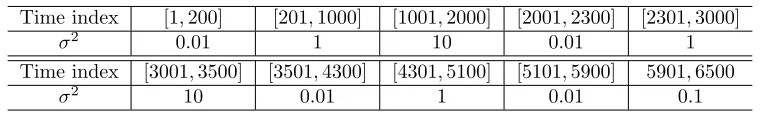
Time index [1,200] [201,1000] [1001,2000] [2001,2300] [2301,3000]
σ2 0.01 1 10 0.01 1
Time index [3001,3500] [3501,4300] [4301,5100] [5101,5900] 5901,6500
σ2 10 0.01 1 0.01 0.1
Table 1: Intervals and {σ2} for synthetic dataset.
AdaMKL: the adaptive version of OMKL that operates in a similar fashion as Algorithm
2, but instead of using our Raker as an ensemble, it adopts OMKL as an instance AI.
Note that AdaMKL, OMKL-B, and M-Forgetron have not been formally proposed in existing works, but we introduced them here only for comparison purposes. All the con-sidered MKL approaches use a dictionary of Gaussian kernels with σ2 = {0.1,1,10}, and AvgMKL, OMKL, AdaMKL, OMKL-B, and M-Forgetron also include a linear, and a poly-nomial kernel with order of 2 into their kernel dictionary. For all MKL approaches, the stepsize for updating kernel combination weights in (21) is chosen as 0.5 uniformly, while the stepsize for updating per-kernel function estimators will be specified later in each test. The regularization parameter is set equal toλ= 0.01 for all approaches. Entries of{xt}and
{yt}are normalized to lie in [0,1]. Regarding AdaMKL and AdaRaker, multiple instances
are initialized on intervals with length |I| := 20,21,22, . . ., along with the corresponding learning rate on the interval I asη(I) := min{1/2,10/p|I|}; see the example in Figure 2. All the results in the tables were reported using the performance at the last time index.
5.1. Synthetic data tests for regression
This subsection presents the synthetic data tests for regression.
Data generation. In this test, two synthetic datasets were generated as follows. For Dataset 1, the feature vectors {xt ∈ R10}14,000
t=1 are generated from the standardized
Gaussian distribution, while yt is generated as yt = Ptτ=1ατκτ(xt,xτ), where {αt} is
generated asαt= 1 +et withet∼ N(0, σα2) andσα= 0.01, while{κt} are kernel functions
that change overtime: fort∈[1,8000]S
[18001,26000],κtis a Gaussian kernel withσ2 = 1,
while for t∈[8001,18000]S
[26001,36000] the Gaussian kernel has σ2 = 10. Therefore, the underlying nonlinear relationship betweenxtand ytundergoes intermittent changes, which
come from corresponding changes in the optimal kernel combinations.
Dataset 2 is generated with more variance and switching points. Specifically, the feature vectors are generated from the standardized Gaussian distribution, while ytis generated as
yt=Ptτ=1ατκτ(xt,xτ), where{κt} change over 10 intervals with differentσ2; see Table 1.
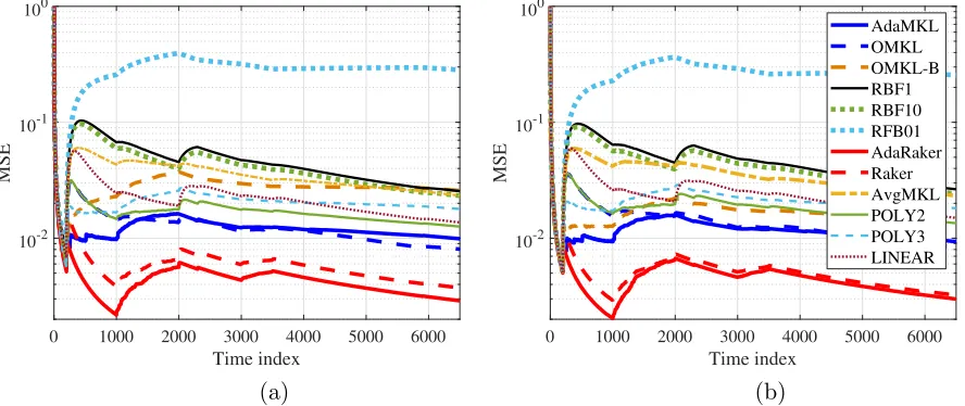
Testing performance. The performance of all schemes is tested in terms of the mean-square (prediction) error MSE(t) := (1/t)Pt
τ=1(yτ−yˆτ)2 in Figure 3 and Figure 4, and
their CPU time is listed in Table 2. For OMKL-B,B = 20 and 50 most recent data samples
were kept in the budget; and for RF-based Raker and AdaRaker approaches, D= 20 and
50 orthogonal random features were used by default. The default stepsize is chosen as
1/√T for RBF, POLY, LINEAR, AvgMKL, OMKL, OMKL-B and Raker. In both tests,
AdaRaker outperforms the alternatives in terms of MSE, especially when the true nonlinear
relationship betweenxtand ytchanges; e.g., compare the MSE of KL-RBF and Raker with
0 0.5 1 1.5 2 2.5 3 3.5
Time index 104
10-3 10-2 10-1 100
MSE
0 0.5 1 1.5 2 2.5 3 3.5
Time index 104
10-3 10-2 10-1 100
MSE
AdaMKL OMKL OMKL-B RBF1 RBF10 RBF01 AdaRaker Raker AvgMKL POLY2 POLY3 LINEAR
(a) (b)
Figure 3: MSE performance on synthetic Dataset 1: a) D=B= 20; b) D=B = 50.
0 1000 2000 3000 4000 5000 6000
Time index
10-2 10-1 100
MSE
0 1000 2000 3000 4000 5000 6000
Time index
10-2
10-1
100
MSE
AdaMKL OMKL OMKL-B RBF1 RBF10 RFB01 AdaRaker Raker AvgMKL POLY2 POLY3 LINEAR
(a) (b)
Figure 4: MSE performance on synthetic Dataset 2: a) D=B= 20; b) D=B = 50.
in Figure 4. This corroborates the effectiveness of the novel AdaRacker method that can flexibly select learning rates according to the variability of the environments, and adaptively combine multiple kernels when the optimal underlying nonlinear relationship is varying over time. In addition, MKL approaches including our Raker approach enjoy lower MSE than that of the single-kernel approaches as well as the simple AvgMKL approach, which is also aligned with our design principle of developing MKL schemes that broaden generalizability of a kernel-based learner over a larger function space.
Dataset 1 Dataset 2
Setting D=B = 20 D=B= 50 D=B= 20 D=B= 50
AdaMKL 318.52 27.29
OMKL 157.10 5.47
RBF 47.83 1.06
POLY2 6.01 0.47
POLY3 28.27 1.24
LINEAR 4.80 0.35
AvgMKL 144.85 5.02
OMKL-B 3.75 4.05 0.72 0.77
Raker 1.39 1.53 0.18 0.20
AdaRaker 21.94 24.24 3.32 3.54
Table 2: CPU time (in seconds) on synthetic datasets. RBF, POLY represents all single-kernel methods using RBF and polynomial single-kernels, since they have the same CPU time.
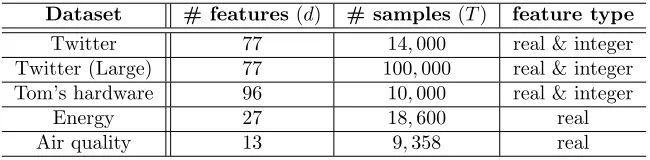
Dataset # features (d) # samples(T) feature type Twitter 77 14,000 real & integer Twitter (Large) 77 100,000 real & integer Tom’s hardware 96 10,000 real & integer
Energy 27 18,600 real
Air quality 13 9,358 real
Table 3: A summary of real datasets used in the tests.
a budget size B = 20 or B = 50 is relatively low, OMKL-B does not perform as well as
AdaRaker and Raker algorithms. Therefore, the AdaRaker and Raker approaches attain a sweet-spot in the performance-complexity tradeoff.
5.2. Real data tests for online regression
To further evaluate our algorithms in real-world scenarios, the present subsection is devoted to testing and comparing on several popular real datasets.
Datasets description. Performance is tested on benchmark datasets from UCI machine learning repository (Lichman, 2013).
• Twitterdataset consists ofT = 14,000 samples from a popular micro-blogging plat-form Twitter, where xt∈R77 include features such as the number of new interactive authors, and the length of discussion on a given topic, whileytrepresents the average
number of active discussion (popularity) on a certain topic (Kawala et al., 2013). A
larger dataset with T = 100,000 is also included for testing only (Ada)Raker and
OMKL-B, since other methods do not scale to such a largeT.
• Tom’s hardwaredataset contains T = 10,000 samples from a worldwide new tech-nology forum, where a 96-dimensional feature vector includes the number of discus-sions involving a certain topic, whileytrepresents the average number of display about
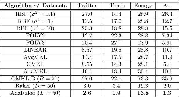
Algorithms/ Datasets Twitter Tom’s Energy Air RBF (σ2= 0.1) 27.0 14.4 28.9 26.3
RBF (σ2= 1) 13.5 17.0 28.8 12.7 RBF (σ2= 10) 23.3 18.8 28.8 15.5 POLY2 12.7 22.3 28.8 7.34 POLY3 20.4 22.7 28.9 5.91 LINEAR 8.57 19.5 28.8 10.7 AvgMKL 14.4 17.5 28.7 11.9
OMKL 8.55 14.3 28.1 6.4
AdaMKL 16.1 18.4 30.4 10.1 OMKL-B (B= 50) 27.0 22.1 73.3 35.9 Raker (D= 50) 3.0 3.4 19.3 2.0 AdaRaker (D= 50) 2.6 1.9 13.8 1.3
Table 4: MSE (10−3) performance of different algorithms with stepsize 1/√T. Algorithms/ Datasets Twitter Tom’s Energy Air
RBF (σ2= 0.1) 17.2 3.3 16.6 8.1 RBF (σ2= 1) 3.3 5.1 16.4 2.8 RBF (σ2= 10) 5.6 13.6 16.4 18.9
POLY2 8.1 15.9 16.2 3.3
POLY3 20.4 20.7 16.2 4.6
LINEAR 2.7 4.8 16.3 2.9
AvgMKL 7.1 6.2 16.3 2.8
OMKL 4.2 3.3 16.2 2.4
AdaMKL 16.1 18.4 30.4 10.1 OMKL-B (B= 50) 9.9 11.8 19 7.1
Raker (D= 50) 2.9 2.6 13.8 1.3 AdaRaker (D= 50) 2.6 1.9 13.8 1.3
Table 5: MSE (10−3) performance of different algorithms with optimally chosen stepsizes.
• energy dataset consists of T = 18,600 samples, with each xt ∈ R27 describing the
humidity and temperature indoors and outdoors, while yt denotes the energy use of
light fixtures in the house (Candanedo et al., 2017).
• air quality dataset collects T = 9,358 instances of hourly averaged responses from five chemical sensors located in a polluted area of Italy. The averaged sensor response
xt ∈ R13 contains the hourly concentrations of e.g., CO, Non Metanic
Hydrocar-bons, and Nitrogen Dioxide (NO2), where the goal is to predict the concentration of polluting chemicals yt in the air (De Vito et al., 2008).
To highlight the effectiveness of our approaches, the datasets mainly include time series data, where non-stationarity is more likely to happen; see Table 3 for a summary.
MSE performance. The MSE performance of each algorithm on the aforementioned
datasets is presented in Table 4. By default, we use the complexity B = D = 50 for
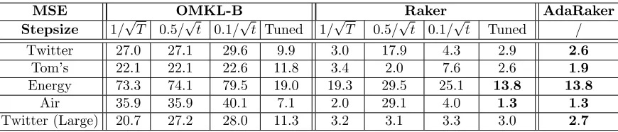
MSE OMKL-B Raker AdaRaker Stepsize 1/√T 0.5/√t 0.1/√t Tuned 1/√T 0.5/√t 0.1/√t Tuned /
Twitter 27.0 27.1 29.6 9.9 3.0 17.9 4.3 2.9 2.6 Tom’s 22.1 22.1 22.6 11.8 3.4 2.0 7.6 2.6 1.9 Energy 73.3 74.1 79.5 19.0 19.3 29.5 25.1 13.8 13.8
Air 35.9 35.9 40.1 7.1 2.0 29.1 4.0 1.3 1.3 Twitter (Large) 20.7 27.2 28.0 11.3 3.2 3.1 3.3 3.0 2.7
Table 6: MSE (10−3) versus the choice of stepsizes with complexity B=D= 50.
OMKL, OMKL-B and Raker. To boost the performance of each algorithm, their MSE when using manually tuned stepsizes is also reported in Table 5, which selects the best stepsize on each dataset among {10−3,10−2,· · ·,103}/√T. A common observation is that leveraging the flexibility of multiple kernels, MKL methods in most cases outperform the algorithms using only a single kernel. By simply averaging over all the kernels, AvgMKL outperforms most of single kernel methods, but performs worse than the adaptive kernel combination methods. This confirms that relying on a pre-selected kernel function is not sufficient to guarantee low fitting loss, while allowing the MKL approaches to select the best kernel combinations in a data-driven fashion holds the key for improved performance.
In most tested datasets, Raker obtains function approximants with lower MSE relative to MKL alternatives without RF approximation. Furthermore, incorporating multiple Raker instances with variable learning rates, AdaRaker consistently yields the lowest MSE in all the tests. As it has been shown in the synthetic data test, the sizable performance gain of AdaRaker appears when the underlying nonlinear models change in the tested time-series datasets. This observation is aligned with our design principle of AdaRaker; that is, when the optimal function predictor varies slowly (fast), AdaRaker tends to select a Raker instance with small (large) learning rate. Interesting enough, even with adaptive learning rate, AdaMKL does not perform as well as OMKL in some tests. This is partially because unlike AdaRaker with fixed number of RFs, each instance in AdaMKL involves
a different number of support vectors (samples). The instance operating on the longest
interval contains at mostT /2 support vectors, which may deteriorate performance relative
to OMKL withT support vectors.
Table 6 further compares the MSE performance of AdaRaker with OMKL-B and Raker using different stepsizes. Clearly, the performance of OMKL-B and Raker is sensitive to the choice of stepsizes. While the optimal stepsize varies from dataset to dataset, selecting
a constant stepsize 1/√T generally leads to better performance than a diminishing one
of O(1/√t). In the online scenarios however, the choice 1/√T may not be feasible if T is unknown ahead of time. In contrast, AdaRaker obtained the best MSE performance without
knowing T, and without the need of stepsize selection, which confirms that AdaRaker is
capable of adapting its stepsize to variable environments with unknown dynamics.
Algorithms/ Datasets Twitter Tom’s Energy Air
RBF 54.7 32.5 26.6 1.71
POLY2 2.25 1.16 2.42 0.58 POLY3 5.62 2.97 7.90 1.51
LINEAR 1.83 0.98 196 0.39
AvgMKL 148.4 81.6 82.4 5.29 OMKL 153.5 81.9 83.3 5.90 AdaMKL 164.1 102.7 117.9 35.3 OMKL-B (B= 50) 1.89 1.42 2.02 0.89 Raker (D= 50) 0.51 0.38 0.65 0.28 AdaRaker (D= 50) 8.64 6.03 10.94 5.28
Table 7: A summary of CPU time (second) on real datasets.
MSE OMKL-B Raker AdaRaker
Complexity 10 50 100 10 50 100 10 50 100 Twitter 28.9 27.0 26.1 5.9 3.0 3.0 3.8 2.6 2.6 Tom’s 22.7 22.1 21.7 8.1 3.4 2.3 7.0 1.9 1.8 Energy 79.1 73.3 67.9 25.7 19.3 16.4 18.7 13.8 13.3 Air pollution 36.7 35.9 35.8 10.1 2.0 1.7 4.3 1.3 1.2 Twitter (Large) 25.0 20.7 19.0 3.9 3.2 3.0 3.3 2.7 2.7
Table 8: MSE (10−3) versus complexity. For OMKL-B, the complexity measure is the data
budget B; and for (Ada)Raker, the complexity measure is the number of RFs D.
2D-dimensional vectors per kernel learner, while the computational complexity of AdaMKL, OMKL, POLY, LINEAR, AvgMKL, and RBF increases with time at least linearly. With a fixed budget size, OMKL-B enjoys light-weight updates that leads to a lower CPU time than alternatives, but higher than Raker. However, given such a limited budget of data, OMKL-B exhibits higher MSE than AdaRaker and Raker; see MSE in Tables 4 and 6.
Running multiple instances of Raker in parallel, the complexity of AdaRaker is reason-ably higher than Raker (roughly logT times higher), but its runtime is still only around 10% of that of AdaMKL, and significantly lower than other single-kernel alternatives especially
when the actual feature dimensiondis higher than the number of random featuresD. The
computational advantage of our MKL algorithms in this test also corroborates the quanti-tative analysis at the end of Section 3.2. Regarding the tradeoff between learning accuracy and complexity, a delicate comparison among OMKL-B, Raker and AdaRaker follows next. Accuracy versus complexity. To further understand the tradeoff between complexity and learning accuracy, the performance of three scalable methods AdaRaker, Raker and
OMKL-B is tested under different parameter settings, e.g., D, the number of random
fea-tures, and B, the number of budgeted data. The MSE performance is reported in Table 8
after one pass of all data in each dataset, while the corresponding CPU time is in Table 9. Not surprising, all three algorithms require longer CPU time as the complexity (in
terms of B or D) increases. For given complexity (same B and D), Raker requires the
Time OMKL-B Raker AdaRaker
Complexity 10 50 100 10 50 100 10 50 100
Twitter 1.42 1.89 2.84 0.42 0.51 0.80 7.58 8.64 11.65 Tom’s 1.00 1.42 2.81 0.41 0.38 0.56 5.09 6.03 8.98 Energy 1.84 2.02 2.32 0.58 0.65 0.76 9.96 10.94 12.47 Air pollution 0.82 0.89 0.97 0.24 0.28 0.32 4.09 5.28 5.29 Twitter (Large) 12.90 16.34 23.6 6.07 6.63 8.42 67.10 78.10 109.40
Table 9: CPU time (second) versus complexity ofB for OMKL-B, and Dfor (Ada)Raker.
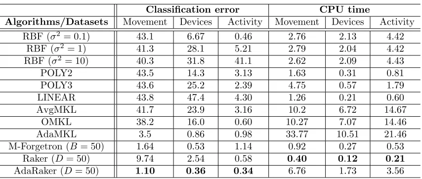
Classification error CPU time
Algorithms/Datasets Movement Devices Activity Movement Devices Activity RBF (σ2= 0.1) 43.1 6.67 0.46 2.76 2.13 4.42
RBF (σ2= 1) 41.3 28.1 5.21 2.79 2.04 4.42 RBF (σ2= 10) 40.3 31.8 41.1 2.62 2.09 4.43
POLY2 43.5 14.3 3.13 1.63 0.31 0.81
POLY3 43.6 25.2 2.39 4.75 0.57 1.79
LINEAR 43.8 47.4 4.30 1.26 0.21 0.60 AvgMKL 41.7 23.9 3.16 10.2 6.72 14.67
OMKL 38.2 16.0 0.60 10.27 7.07 14.46 AdaMKL 3.5 0.86 0.98 33.77 10.51 21.46 M-Forgetron (B= 50) 1.64 0.53 1.14 0.92 0.27 0.53
Raker (D= 50) 9.74 2.54 0.58 0.40 0.12 0.21 AdaRaker (D= 50) 1.10 0.36 0.34 6.76 1.73 3.56
Table 10: Classification error (%) and runtime (second) of different algorithms with the
default stepsize 1/√T for RBF, OMKL and Raker, and with complexity B =D= 50.
remarkable especially in the Energy and Air pollution datasets. For Twitter (Large) dataset,
the performance of AdaRaker does not improve as RFs increase from D= 50 toD= 100,
which implies thatD= 50 is enough to provide reliable kernel approximation in this dataset. Considering that AdaRaker is embedded with concurrent logtRaker instances at timet, its CPU time is relatively higher. However, one would expect a major reduction in the number of concurrent instances and thus markedly lower CPU time, if a larger basic interval size (instead of base number 2 in Figure 2) is incorporated in AdaRaker real implementation.
At this point, one may wonder how many RFs are enough for Raker and AdaRaker to
guarantee the same online learning accuracy as that of OMKL-B with B samples. While
this intriguing question has been recently studied in the batch setting with an answer of
D =O(√B) RFs (Rudi and Rosasco, 2017), its thorough treatment in the online setting
constitutes our future research.
5.3. Real data tests for online classification
perceptron-Classification error Algorithms/Datasets Movement Devices Activity
RBF (σ2= 0.1) 28.9 5.16 0.26 RBF (σ2= 1) 1.27 0.42 0.53 RBF (σ2= 10) 1.10 0.36 1.14
POLY2 8.19 1.7 0.56
POLY3 15.2 17.3 0.45
LINEAR 7.46 30.7 0.60
AvgMKL 1.69 2.26 0.48
OMKL 1.10 0.36 0.29
AdaMKL 3.50 0.86 1.00
M-Forgetron (B= 50) 1.64 0.53 1.14 Raker (D= 50) 1.10 0.28 0.24 AdaRaker (D= 50) 1.10 0.36 0.34
Table 11: Classification error (%) of different algorithms with the dataset-specific optimally
chosen stepsizes for RBF, OMKL and Raker, and with complexity B=D= 50.
based Forgetron algorithm. Kernels and all other parameters such as the default stepsizes, are chosen as those in the regression task.
Datasets description. We test classification performance on the following datasets.
• Movement dataset consists of T = 13,197 temporal streams of received signal strength (RSS) measured between the nodes of a wireless sensor network, with each
xt ∈ R4 comprising 4 anchor nodes (Bacciu et al., 2014). Data has been collected
during user movements at the frequency of 8 Hz (8 samples per second). The RSS samples in the dataset have been rescaled to lie in [−1,1]. The binary label yt
indi-cates whether the user’s trajectory will lead to a change in the spatial context (here a room change) or not.
• Electronic Device dataset consists of T = 3,600 samples collected as part of a government sponsored study called ‘Powering the Nation,’ where the feature vectors xt∈R60represent electricity readings from different households over 15 mins, sampled within a month (Lines et al., 2011). Binary labelyt represents the type of electronic
devices used at the certain interval of time time: dishwasher or kettle.
• Human Activity dataset consists of T = 7,352 samples collected from a group of 30 volunteers wearing a smartphone (Samsung Galaxy S II) on their waist to monitor activities (Anguita et al., 2013). Feature vectors{xt∈R30}here measure e.g., triaxial acceleration and angular velocity, while binary labelyt represents the activity during
a certain period: walking or not walking.
Classification performance. The classification error (1/T)PT
t=1max{0,sign(−ytyˆt)} and the CPU time of each algorithm on these datasets are summarized in Table 10 when
a default stepsize 1/√T is used for POLY, LINEAR, RBF, AvgMKL, OMKL and Raker.
The budget of M-Forgetron is set at B = 50 samples, while Raker and AdaRaker adopt
OMKL Raker AdaRaker Stepsize 1/√T 1/√t 10/√t Tuned 1/√T 1/√t 10/√t Tuned / Movement 38.2 39.5 22.3 1.10 12.1 8.60 1.79 1.10 1.10
Devices 16.0 13.2 6.06 0.36 2.54 2.04 0.53 0.28 0.36 Activity 0.60 0.53 0.50 0.29 0.58 0.52 0.54 0.24 0.34
Table 12: Classification error (%) versus different choices of stepsizes with B=D= 50.
Classification error CPU time
Algorithms/ Datasets Movement Devices Activity Movement Devices Activity M-Forgetron (B= 10) 1.60 0.53 1.14 0.92 0.26 0.53 M-Forgetron (B= 50) 1.64 0.53 1.14 0.92 0.27 0.53 M-Forgetron (B= 100) 1.42 0.53 1.14 0.94 0.29 0.53 Raker (D= 10) 26.3 8.37 3.26 0.35 0.10 0.18 Raker (D= 50) 9.74 2.54 0.58 0.40 0.12 0.21 Raker (D= 100) 4.65 1.53 0.43 0.46 0.15 0.26 AdaRaker (D= 10) 2.46 0.66 0.68 6.13 0.65 3.22 AdaRaker (D= 50) 1.10 0.36 0.34 6.76 1.73 3.56 AdaRaker (D= 100) 1.10 0.36 0.34 7.55 2.04 4.22
Table 13: Classification error (%) and CPU time (second) versus complexity.
classification accuracy and the Raker has the lowest CPU time among all competing algo-rithms. Without having to tune stepsizes, the performance of AdaMKL and M-Forgetron is also competitive in this case. To explore the best performance of each algorithm, the clas-sification performance under manually tuned stepsizes is reported in Table 11, where each algorithm uses the best stepsize among {10−3,10−2,· · · ,103}/√T for each dataset. With the optimally chosen stepsizes, the performance of all algorithms improves, and Raker even achieves slightly lower classification error than AdaRaker in some datasets. This is rea-sonable since compared to Raker with the offline tuned stepsize, AdaRaker will incur some error due to the online adaptation to several (possibly suboptimal) learning rates.
To corroborate the effectiveness of our algorithms in adapting to unknown dynamics
(e.g., unknown time horizon T and variability), Table 12 compares the performance of
AdaRaker with OMKL and Raker using default, diminishing and optimally tuned stepsizes. Similar to regression tests, the performance of Raker and OMKL is sensitive to the step-size choice, while AdaRaker achieves the desired performance by combining learners with different learning rates. By simply averaging over all the kernels, AvgMKL outperforms sin-gle kernel methods in most cases, but performs much worse than OMKL and (Ada)Raker methods. Note that the Raker also achieves competitive classification accuracy when the constant stepsize 1/√T is used. Such a choice is however not always feasible in practice, since it requires knowledge of how many data samples will be available ahead of time. Accuracy versus complexity. In this experiment, we test classification performance in terms of both classification error and CPU time for different levels of complexity; see
Table 13. We use the number of support vectors B for M-Forgetron, and the number of
their performance using the default stepsize. It is expected that CPU time increases as the complexity increases, and the classification error decreases as the complexity grows. For all three datasets, the AdaRaker achieves the lowest classification error, and the Raker outperforms the M-Forgetron while at the same time it is more efficient computationally.
6. Concluding Remarks
This paper dealt with kernel-based learning in environments with unknown dynamics that also include static or slow variations. Uniquely combining advances in random feature based function approximation with online learning from an ensemble of experts, a scalable online multi-kernel learning approach termed Raker, was developed for static environments based on a dictionary of kernels. Endowing Raker with capability of tracking time-varying optimal function estimators, AdaRaker was introduced as an ensemble version of Raker with variable learning rates. The key modules of the novel learning approaches are: i) the random features are for scalability, as they reduce the per-iteration complexity; ii) the preselected kernel dictionary is for flexibility, that is to broaden generalizability of a kernel-based learner over a larger function space; iii) the weighted combination of kernels adjusted online accounts for the reliability of learners; and, iv) the adoption of multiple learning rates is for improved adaptivity to changing environments with unknown dynamics.
Complementing the principled algorithmic design, the performance of Raker is rigor-ously established using static regret analysis. Furthermore, without a-priori knowledge of dynamics, it is proved that AdaRaker achieves sub-linear dynamic regret, provided that either the loss or the optimal learning function does not change on average. Experiments on synthetic and real datasets validate the effectiveness of the novel methods.
Acknowledgments
This work is supported in part by the National Science Foundation under Grant 1500713 and 1711471, and NIH 1R01GM104975-01. Yanning Shen is also supported by the Doctoral Dissertation Fellowship from the University of Minnesota.
Appendix A. Proof of Lemma 1
To prove Lemma 1, we introduce two intermediate lemmata as follows.
Lemma 3 Under (as1), (as2), and fˆp∗ as in (26) with Fp := {fˆp|fˆp(x) = θ>zp(x),∀θ ∈
R2D}, let{fˆp,t(xt)} denote the sequence of estimates generated by Raker with a pre-selected
kernel κp. Then the following bound holds true w.p.1
T
X
t=1
Lt( ˆfp,t(xt))− T
X
t=1
Lt( ˆfp∗(xt))≤
kθ∗pk2
2η +
ηL2T
2 (42)
Proof: Similar to the regret analysis of online gradient descent (Shalev-Shwartz, 2011), using (12) for any fixedθ, we find
kθp,t+1−θk2 =kθp,t−η∇L(θ>p,tzp(xt), yt)−θk2 (43)
=kθp,t−θk2+η2k∇L(θ>p,tzp(xt), yt)k2−2η∇>L(θ>p,tzp(xt), yt)(θp,t−θ).
Meanwhile, the convexity of the loss under (as1) implies that
L(θ>p,tzp(xt), yt)− L(θ>zp(xt), yt)≤ ∇>L(θ>p,tzp(xt), yt)(θp,t−θ). (44)
Plugging (44) into (43) and rearranging terms yields
L(θ>p,tzp(xt), yt)−L(θ>zp(xt), yt)≤
kθp,t−θk2− kθp,t+1−θk2
2η +
η
2k∇L(θ >
p,tzp(xt), yt)k2.
(45) Summing (45) over t= 1, . . . , T, with ˆfp,t(xt) =θ>p,tzp(xt), we arrive at
T
X
t=1
L( ˆfp,t(xt), yt)−L(θ>zp(xt), yt)
≤kθp,1−θk 2− kθ
p,T+1−θk2
2η +
η
2
T
X
t=1
k∇L(θ>p,tzp(xt), yt)k2 (a)
≤ kθk 2
2η +
ηL2T
2 (46)
where (a) uses the Lipschitz constant in (as2), the non-negativity of kθp,T+1−θk2, and the initial value θp,1 =0. The proof of Lemma 3 is then complete by choosing θ = θ∗p =
PT
t=1α∗p,tzp(xt) such that ˆfp∗(xt) =θ>zp(xt) in (46).
Lemma 3 establishes that the static regret of the Raker is upper bounded by some constants,
which mainly depend on the stepsize in (19) and the time horizon T.
In addition, we will bound the difference between the loss of the solution obtained from Algorithm 1 and the loss of the best single kernel-based online learning algorithm. Specifically the following lemma holds:
Lemma 4 Under (as1) and (as2), with {fˆp,t} generated from Raker, it holds that
T
X
t=1 P
X
p=1 ¯
wp,tLt( ˆfp,t(xt))− T
X
t=1
Lt( ˆfp,t(xt))≤ηT +
lnP
η (47)
where η is the learning rate in (21), and P is the number of kernels in the dictionary.
Proof: LettingWt:=PPp=1wp,t, the weight recursion in (21) implies that
Wt+1 =
P
X
p=1
wp,t+1 = P
X
p=1
wp,texp
−ηLtfˆp,t(xt)
≤
P
X
p=1
wp,t
1−ηLt
ˆ
fp,t(xt)
+η2Lt
ˆ
fp,t(xt)
2