ISSN: 2231-5373
http://www.ijmttjournal.org
Page 232
Analysis of Two-Dissimilar Component
System with Uncertain Availability of
Repairman
Praveen Gupta #1 and Ruchi Yadav#2
School of studies in statistics Vikram University, Ujjain (M. P.) India.
Abstract
The system consists of a two-dissimilar components working in parallel, say A and B. Both the components are operative initially at time t=0. A single repair facility is available for the repair. Upon failure of a component the repair facility, if not busy, is available with some fixed probability p. If repair facility is not available at the time of a failure of a component, it is called for repair. The repair facility appearance time distribution is exponential. When repair facility is busy in repair of the failed component, the other failed component waits for its repair. After repair, the components become as good as new. The repair time of both the components are arbitrary functions of time. Failure time distributions are assumed to be exponential.
Key words: Reliability, Mean time to system failure, Availability, Exponential distribution.
Introduction
Two-unit standby redundant systems have been extensively studied by several authors in the past. Said and Sherbeny (2010) analyzed a two-unit cold standby system with two stage repair and waiting time. In this paper a two dis-similar component system is considered. The system operates even if a single component operates. A single repair facility is available with some fixed probability for the repair of failed components.
System Assumption and Description
The system consists of a two-dissimilar components working in parallel, say A and B. Both the components are operative initially at time t=0. A single repair facility is available for the repair. Upon failure of a component the repair facility, if not busy, is available with some fixed probability p. If repair facility is not available at the time of a failure of a component, it is called for repair. The repair facility appearance time distribution is exponential. When repair facility is busy in repair of the failed component, the other failed component waits for its repair. After repair, the components become as good as new. The repair time of both the components are arbitrary functions of time. Failure time distributions are assumed to be exponential. Several measures of system effectiveness such as MTSF, A, B etc. are obtained by using regenerative point technique.
Notations and States of the System
E set of regenerative states {S0, S1, S2, S4, S6 }
E
set of non-regenerative states {S3, S4} failure rate of component A.
failure rate of component B.
rate of appearance of repair facility.
f(.) Pdf of repair rate of component A.
g(.) Pdf of repair rate of component B.
p = (1–q)=probability that the repairman is available for repairs.
The system may be in one of the following states:
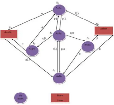
S0 (ANBN) The components A and B both are in normal operative mode.
S1 (AFBN) Failed component A is waiting for repair and component B is operative.
S3 (ARBN) Component A is under repair and B is operative.
S4 (ANBR) Component A is in operative mode and component B is under repair.
ISSN: 2231-5373
http://www.ijmttjournal.org
Page 233
S6(ARBWR) Component A is under repair and component B waits for its repair.
Figure 1 Analysis of two dissimilar component with uncertain availability of repairman+
Transition Probabilities and Sojourn Times
Let T0 (=0), T1, T2 … be the epochs at which the system enters the state SiE, and
Let Xn denotes the state entered at epoch Tn+1, i.e. just after the transition at Tn. Then
{Xn, Tn} constitutes a Markov-renewal process with the state space E and
Qij(t) = Pr[Xn+1 = Sj | Tn+1 – Tn t|xn = Si].
The transition probability matrix of the embedded Markov chain is:
P = (pij) = { ij
t
Q
(t)} = {Qij ()}.
By simple probabilistic considerations, the non-zero elements of Q = {Qij(t)} can be obtained as follows: For the
system to reach state S1 from S0 on or before time t, we suppose that the system transits from S0 to S1 during (u, u+du); u t while it does not transits to any of the state‟s S2, S3 and S4 up to the time u. The probability of
this event is:
qe-udu.(p + q)e-u = qe-udu.
Since u varies from 0 to 1, therefore
Q01(t) =
t
( )u
0
q e
du
Taking limit t tends to infinity, we have
ij t ij
p
limQ (t).
The non-zero elements of pij are given below:
01
ISSN: 2231-5373
http://www.ijmttjournal.org
Page 234
03
p
p /
,
p
04
p /
,
13
p
/
,
p
16
/
,
24
p
/
,
p
25
/
,
30
p
F
,
p
(6)34
1 F
p ,
36
40
p
G
,
(5)
43 45
p
1 G
p .
We observe the following relationships among the above study state probabilities:
01 02 03 04
p
p
p
p
1,
13 16
p
p
1,
24 25
p
p
1,
6
30 36 36 34
p
p
p
p
1,
(5)
40 45 40 43
p
p
p
p
1.
Mean sojourn timei in state Si is defined as the time that the system continues in state Si before
transiting to any state. If T denotes the sojourn timein Si theniin Si is:- i
0
E(T)
P(T t)dt
.Using this we can obtain the following expressions,
t
0 0
e
dt 1/
,
t
1 0
e
dt 1/
,
t
2 0
e
dt 1/
,
3 0
F(t)dt,
4 0
G(t)dt.
In terms of Laplace-Stieltje‟s transform of Qi (t), we define mij as follows:-
ijij ij s 0
d
m
Q (0) lim
Q (s).
ds
s u
01
0
Q (s)
q e
du q / s
,
s u
02
0
Q (s)
q e
du q / s
,
s u
03
0
Q (s)
p e
du p / s
,
ISSN: 2231-5373
http://www.ijmttjournal.org
Page 235
s u
04
0
Q (s)
p e
du p / s
,
s u
13
0
Q (s)
e
du
/ s
,
s u
16
0
Q (s)
e
du
/ s
,
s u
24
0
Q (s)
e
du
/ s
,
s u *
30
0
Q (s)
e
dF(u)
F
s ,
s u *
40
0
Q (s)
e
dG(u)
G
s ,
(6) st
t
* *34
0
Q (s)
e
1 e
dF(t), f (s) f (s
)
(5) st
t
* *43
0
Q (s)
e
1 e
dG(t), g (s) g (s
).
We have,
'
201 01
m
Q (s) q /
,
02
' 2
02
m
Q (0) q /
,
03
' 2
03
m
Q (0) p /
,
04
' 2
04
m
Q (0) p /
,
13
' 2
13
m
Q (0)
/
,
16
' 2
16
m
Q (0)
/
,
24
' 2
24
m
Q (0)
/
,
25
' 2
25
m
Q (0)
/
,
'(6)(6) t t
34 34
0 0
m
Q (0)
te dF(t)
te E(t)dt,
'(5)(5) t t
43 43
0 0
m
Q (0)
te dG(t)
te G(t)dt,
' t30 30
0
m
Q (0)
te dF(t),
ISSN: 2231-5373
http://www.ijmttjournal.org
Page 236
' t40 40
0
m
Q (0)
te dG(t).
It can be easily seen that,
01 02 03 04 0
m
m
m
m
,
16 13 1
m
m
,
24 25 2
m
m
,
(6)
30 34 3
m
m
,
(5)
40 43 4
m
m
.
Reliability and Mean Time to System Failure (MTSF)
Let the random variable Ti be the time to system failure (TSF) when the system starts its operation
from SiE, then the reliability of the system is given by,
Ri(t) = P (Ti> t).
In order to determine Ri(t), we regard the failed states S5, S6 of the system as absorbing states. By
simple probabilistic reasoning, we observe that
R (t)
0 is the sum of following contingencies:(i) System remains up in state S0 without making any transition to any other state up to time t. The
probability of this contingency is,
t 0
e
z (t).
(ii) System first enters the regenerative state S1 during (u, u+du), u t and then starting from S1, it remains up without any break down for the time
duration (t – v). The probability of this contingency is,
t
01 1 01
0
q (u)duR (t u) q (t)
© R1(t).(iii) System first enters the regenerative state S2 during (u, u+du), u t and then starting from S2, it remains up without any breakdown for the time
duration (t – v). The probability of this contingency is,
t
02 2 02
0
q (u)duR (t u) q (t)
© R2(t).(iv) System first enters the regenerative state S3 during (u, u+du), u t and then starting from S3, it remains up without any breakdown for the time duration
(t – v). The probability of this contingency is,
t
03 3 03
0
q (u)duR (t u) q (t)
ISSN: 2231-5373
http://www.ijmttjournal.org
Page 237
(v) System first enters the regenerative state S4 during
(u, u+du); u t and then starting from S3, it remains up without any breakdown for the time duration
(t – v). The probability of this contingency is,
t
04 4 04
0
q (u)duR (t u) q (t)
© R4(t).Thus,
R0(t) = Z1(t) + q13(t) © R3(t)
Similarly,
R1(t) = Z1(t) + q13(t) © R3(t)
R2(t) = Z2(t) + q24(t) © R4(t)
R3(t) = Z3(t) + q30(t) © R0(t)
R4(t) = Z4(t) + q40(t) © R0(t),
Where,
t 0
Z (t) e
,
t 1Z (t) e
,
t 2
Z (t) e
,
t3
Z (t) e F(t),
t 4
Z (t) e G(t).
For brevity, we have omitted the argument„s‟ from
q (s),
*ijZ (s)
*i andR (s)
*i . Solving the above equation for *0
R (s)
, we get* 1
0
1
N (s)
R (s)
,
D (s)
Where,
N (s)
1
Z
0*
q Z
*01 1*
q q
01 13* *
q
02*
Z
2*
q Z
24* *4
* * *
* * *
01 13 24 3 34 4
q q
q
Z
q Z
* * * * * * * * *
1 01 13 30 02 24 03 30 04 40
D (s)
1 q q q
q q
q q
q q
.
Taking the inverse Laplace transform (ILT) of the above equation, we can get the reliability of the system when it starts from state S0, the mean time to system failure (MTSF) can be obtained on using the
formula
0 00
E T
R (t)dt
* 0 s 0
limR (s)
1
1
N (0)
.
D (0)
ISSN: 2231-5373
http://www.ijmttjournal.org
Page 238
To determine N1 (0) and D1 (0), we must first obtain* i
Z (s),
using the result*
i i
s 0
0
lim Z (s)
Z (t)dt.
Therefore,
*
0 0
Z (0)
,
Z (0)
1*
1,
*
2 3
Z (0)
,
Z (0)
*4
4.
Thus, using
q (0) p
*ij
ij and aboveZ (s)
*i , we get,
1 0 01 1 01 13 02 2 24 4
N (0)
p
p p
p
p
p p
01 13p
24
3p
34 4
And,
D (0)
1
1 p p p
01 13 30
p p
02 24
p p
03 30
p p
04 40
.
Availability Analysis
Let
A (t),
11A (t)
12 andA (t)
13 be the probabilities that the system is up at epoch t due to first component, due to second component and due to both the components in parallel respectively when initially system starts from SiE.Using simple probabilistic laws it can be seen that A0 (t) is the sum of the following probabilities of
mutually exclusive contingencies.
(i) The system does not transits to state S0 till time t. The probability of this event is
t 0
e
Z (t).
(ii) The system transits to S1 from S0 in (u, u+du); u t and then starting from S1, it is observed to be up
at epoch t, with probability A1(t – u). Therefore
t
01 1
0
q (u)duA (t u).
(iii) The system transits to S2 from S0 in (u, u+du); u t and then starting from S2, it is observed to be up
at epoch t, with probability A2(t – u). Therefore,
t
02 2
0
q (u)duA (t u).
(iv) The system transits to S3 from S0 in (u, u+du); u t and then starting from S3, it is observed to be up
at epoch t, with probability A3(t – u). Therefore
t
03 3
0
q (u)duA (t u).
(v) The system transits to S4 from S0 in (u, u+du); u t and then starting from S4, it is observed to be up
ISSN: 2231-5373
http://www.ijmttjournal.org
Page 239
t
04 4
0
q (u)duA (t v).
Taking Laplace Transform (L.T.) of the above relation and writing the resulting set of equation in the matrix form, we get
0
1
2
3
4
5
6
1
1 *
0 01 02 0
1 *
13
1 * * *
24 25 2
1 * 6*
30 34
* (5)* *
1
40 43 4
*
1 53
*
1 64
A
q
q
q
0
0
0 0
Z
A
0
0
0
q
0
0 0
0
A
0
0
1
0
q
q
0
Z
A
q
0
0
0
q
0 0
0
.
q
0
0
q
1
0 0
Z
A
0
0
0
q
0
0 0
0
A
0
0
0
0
q
0 0
0
A
For brevity, the argument„s‟ has been omitted from
q (s),
*ijA (s)
1*i andZ (s)
1* . Solving the abovematrix for
A (s)
'*0 , we get, '*0 2 2
A (s) N (s)/D (s),
Where
N (s)
2
Z
*0
q Z
02 2* *
1 q Z
34* 43*
q
01
q q
13 34
q
16
And,
* *
* *
* * * *
* * *2 34 43 01 10 01 13 24 43 30 03 30
D (s) 1 q q
1 q q
q q
q q q
q q
* * * * * * * * * * * *
04 53 64 30 01 13 34 13 40 04 64 53
q q q q
q
q q
q
q
q q q
*
* * * *
34 03 04 53 64 40
q
q
q q q
q .
Now to obtain the steady-state probabilities that the system will be operative due to first component, we proceed as follows –
*
i i i
Z (0)
Z (t)dt
(i = 0, 2, 4)and using the result
q (0) p
*ij
ij, we have
2 34 43 10 01 01 13 24 43 30 03 30
D (0) 1 p p 1 p p
p p
p p p
p p
p p p p
04 53 64 30
p
01p p
13 34
p
13p
40
p p p
04 64 53
p
34p
03
p p p
04 53 64p
40
1 p p
34 43
p p
01 10
p p p p
01 10 34 43
p p p
01 13 30
p p p p
01 24 43 30ISSN: 2231-5373
http://www.ijmttjournal.org
Page 240
1 p p
01 03p
04p p 1 p p
34 43
01 03p
04
p p p
02 10
13
p p p
02 34 43p
10
p
13
p
02
p p p
34 43 02
p
02
p p p
02 34 43
0.
Therefore, the steady -state probability that the system will be operative due to first component is given by
,
' '
0 t 0
A
lim A (t)
*
20
s 0 s 0
2
N (s)
limsA (t) lims
D (s)
2' 2
N (0)
,
D (0)
as D2(0) = 0.Similarly, the steady state probabilities that the system will be operative due to second component,
2 2
0 t 0
A
lim A (t)
2* 3
0 '
s 0 s 0
2
N (s)
limsA (s) lims
D (s)
3' 2
N (0)
,
D (0)
as D2(0) = 0.
3 3
0 t 0
A
lim A (t)
3*
40 '
s 0 s 0
2
N (s)
limsA (t) lims
D (s)
4' 2
N (0)
,
D (0)
as D2(0) = 0,Where,
2 0 02 2 34 43 01 13 34 16
N (0)
p
1 p p
p
p p
p
p p
02 24
p p p
25 64 53
p p
34 03
p
04
p p p
43 53 64
4
3 0 01 13 43 64 02 24 43 25 34
N (0)
p
p
p p
p
p p
p p
p p
03 30 3
1 13p
p p
04 40
p p
03 30And,
4 01 34 43 1 02 24 40 2
ISSN: 2231-5373
http://www.ijmttjournal.org
Page 241
To obtainD (0)
'2 , we collect the coefficient of
q (0)
ij*
m
ij
inD (0)
'2 for various values of i and j as follows –Coefficient of
m
01
1 p p
34 43
p
10
p
13
p
43
p
30
p p
13 34
p
24
p
40
1 p p p
34 43 10
p
13
p
16p
30
p
40
p p
30 40
1 p p
34 43p
10
p
13
p
161 p p
34 43
1 p p
34 43Coefficient of
m
02
p p
24 43
p p
25 64
p
30
p
24
p p p
25 64 34
p
40
1 p p
34 43Coefficient of
m
03
p
30
p p
34 40
1 p p
34 43Conclusion
This paper describes an improvement over the Said and Sherbeny (2010).They analyzed a two-unit cold standby system with two stage repair and waiting time. In this paper we analyzed a two dis-similar component system. The system operates even if a single component operates. A single repair facility is available with some fixed probability for the repair of failed components. . Several measures of system effectiveness such as MTSF,
A,B etc. are obtained by using regenerative point technique which shows that the proposed model is better than Said and Sherbeny (2010).
Acknowledgement
It is with the grace of almighty God that I have been able to complete this paper and again pray him that my efforts may not go in vain. I am also highly thankful to Dr. H. P. Singh and Dr. Rajesh Tailor for stimulating and co-operating me throughout the work.
References
[1] Goel, L.R. and Gupta, P. (1983): „Stochastic behavior of a two unit (dissimilar) hot standby system with three modes‟. Microelectron and Reliability, 23, 1035-1040.
[2] Gupta, P. and Saxena, M., (2006): “Reliability analysis of a single unit and two protection device system with two types of failure.” Ultra Science 18, 149-154.
[3] Mogha, A.K. and Gupta, A.K., (2002): „A two priority unit warm standby system model with preparation of repair‟. The Aligarh Journal of Statistics, 22, 73-90 (2002).