Scaling Up Sparse Support Vector Machines by Simultaneous Feature and Sample Reduction

(1)

Scaling Up Sparse Support Vector Machines by

Simultaneous Feature and Sample Reduction

Bin Hong∗ [email protected]

State Key Lab of CAD&CG, College of Computer Science, Zhejiang University Hangzhou, 310058, China

Weizhong Zhang∗ [email protected]

Tencent AI Lab, Shenzhen, 518000, China

Wei Liu [email protected]

Tencent AI Lab, Shenzhen, 518000, China

Jieping Ye [email protected]

Department of Computational Medicine and Bioinformatics, University of Michigan Ann Arbor, MI, 48104-2218, USA.

Deng Cai† [email protected]

Xiaofei He [email protected]

Jie Wang [email protected]

Department of Electronic Engineering and Information Science University of Science and Technology of China, Hefei, 230026, China

Editor:Sanjiv Kumar

Abstract

Sparse support vector machine (SVM) is a popular classification technique that can si-multaneously learn a small set of the most interpretable features and identify the support vectors. It has achieved great successes in many real-world applications. However, for large-scale problems involving a huge number of samples and ultra-high dimensional features, solving sparse SVMs remains challenging. By noting that sparse SVMs induce sparsities in both feature and sample spaces, we propose a novel approach, which is based on accurate estimations of the primal and dual optima of sparse SVMs, to simultaneously identify the inactive features and samples that are guaranteed to be irrelevant to the outputs. Thus, we can remove the identified inactive samples and features from the training phase, leading to substantial savings in the computational cost without sacrificing the accuracy. Moreover, we show that our method can be extended to multi-class sparse support vector machines. To the best of our knowledge, the proposed method is thefirst staticfeature and sample reduction method for sparse SVMs and multi-class sparse SVMs. Experiments on both synthetic and real data sets demonstrate that our approach significantly outperforms state-of-the-art methods and the speedup gained by our approach can be orders of magnitude.

Keywords: screening, SVM, dual problem, optimization, classification

∗. The first two authors contribute equally. †.Corresponding author.

c

(2)

1. Introduction

Sparse support vector machine (SVM) (Bi et al., 2003; Wang et al., 2006) is a powerful technique that can simultaneously perform classification by margin maximization and variable selection via`1-norm penalty. The last few years have witnessed many successful applications of sparse SVMs, such as text mining (Joachims, 1998; Yoshikawa et al., 2014), bioinformatics (Narasimhan and Agarwal, 2013), and image processing (Mohr and Obermayer, 2004; Kotsia and Pitas, 2007). Many algorithms (Hastie et al., 2004; Fan et al., 2008; Catanzaro et al., 2008; Hsieh et al., 2008; Shalev-Shwartz et al., 2011) have been proposed to efficiently solve sparse SVM problems. However, the applications of sparse SVMs to large-scale learning problems, which involve a huge number of samples and extremely high-dimensional features, still remain challenging.

An emerging technique, called screening (El Ghaoui et al., 2012), has been shown to be promising in accelerating the training processes of large-scale sparse learning models. The essential idea of screening is to quickly identify the zero coefficients in the sparse solutions without solving any optimization problems such that the corresponding features or samples—that are calledinactive features or samples—can be removed from the training phase. Then, we only need to perform optimization on the reduced data sets instead of the full data sets, leading to a substantial saving in the computational cost. Here, we need to emphasize that screening differs greatly from feature selection, although they look similar at the first glance. To be precise, screening is devoted to accelerating the training processes of many sparse models including Lasso, sparse SVMs, etc., while feature selection is the goal of these models. In the past few years, many screening methods are proposed for a large set of sparse learning techniques, such as Lasso (Tibshirani et al., 2012; Xiang and Ramadge, 2012; Wang et al., 2015), group Lasso (Ndiaye et al., 2016),`1-regularized logistic regression (Wang et al., 2014b), and SVMs (Ogawa et al., 2013). Most of the existing methods are in the same framework, i.e., estimating the optimum of the dual (resp. primal) problem and then developing the screening rules based on the estimations to infer which components of the primal (resp. dual) optimum are zero from the KKT conditions. The main differences among them are the techniques they use to develop their optima estimations and rules and the different sparse models they focus on. For example, SAFE (El Ghaoui et al., 2012) estimates the dual optimum by calculating the optimal value’s lower bound of the dual problem. The Lasso screening method (Wang et al., 2015) estimates the optimum based on the non-expensiveness (Bauschke et al., 2011) of the projection operator by noting that its dual problem boils down to finding the projection of a given point on a convex set. Moreover, a screening method is called static if it triggers its screening rules before training, and

dynamic if during the training process. Empirical studies indicate that screening methods

can lead to orders of magnitude of speedup in computation time.

(3)

models with largenandp. We cannot address this problem by simply combining the existing feature and sample screening methods either. The reason is that they could mistakenly discard relevant data as they are specifically designed for different sparse models. Recently, Shibagaki et al. (2016) considered this issue and proposed a method to simultaneously identify the inactive features and samples in a dynamic manner, and they trigger their testing rule when there is a sufficient decrease in the duality gap during the training process. Thus, the method in Shibagaki et al. 2016 can discard more and more inactive features and samples as the training proceeds and one has small-scale problems to solve in the late stage of the training process. Nevertheless, the overall speedup is limited as the problems’ size can be large in the early stage of the training process. To be specific, the method in Shibagaki et al. 2016 depends heavily on the duality gap during the training process. The duality gap in the early stage can always be large, which makes the dual and primal estimations inaccurate and finally results in ineffective screening rules. Hence, it is essentially solving a large problem in the early stage. This will be verified in the experimental comparisons in Section 6 and similar results can also be found in the recent work (Massias et al., 2018), which merely focuses on Lasso.

In this paper, to address the limitations in the dynamic screening method, we propose a novel screening method that can Simultaneously identify Inactive Features and Samples (SIFS) for sparse SVMs in a static manner, and we only need to perform SIFS once before

(instead of during) training. Thus, we only need to run the training algorithm on small-scale problems. The major technical challenge in developing SIFS is that we need to accurately estimate the primal and dual optima. The more accurate the estimations are, the more effective SIFS is in detecting inactive features and samples. Thus, our major technical contribution is a novel framework, which is based on the strong convexity of the primal and dual problems of sparse SVMs for deriving accurate estimations of the primal and dual optima (see Section 3). Another appealing feature of SIFS is the so-calledsynergistic effect

(Shibagaki et al., 2016). Specifically, the proposed SIFS consists of two parts, i.e., Inactive Feature Screening (IFS) andInactiveSampleScreening (ISS). We show that discarding inactive features (resp. samples) identified by IFS (resp. ISS) leads to a more accurate estimation of the primal (resp. dual) optimum, which in turn dramatically enhances the capability of ISS (resp. IFS) in detecting inactive samples (resp. features). Thus, SIFS applies IFS and ISS in an alternating manner until no more inactive features and samples can be identified, leading to much better performance in scaling up large-scale problems than the application of ISS or IFS individually. Moreover, SIFS (see Section 4) is safe in the sense that the detected features and samples are guaranteed to be absent from the sparse representations. To the best of our knowledge, SIFS is the first static screening rule for sparse SVMs, which is able to simultaneously detect inactive features and samples. Experiments (see Section 6) on both synthetic and real data sets demonstrate that SIFS significantly outperforms the state-of-the-art (Shibagaki et al., 2016) in improving the training efficiency of sparse SVMs and the speedup can be orders of magnitude.

(4)

SIFS we developed for sparse SVMs is mainly based on the strong convexity of the primal and dual problems. Therefore, the idea of SIFS is also applicable for multi-class sparse SVMs. Experimental results show that the speedup gained by SIFS in multi-class sparse SVMs can also be orders of magnitude.

For the convenience of presentation, we postpone the detailed proofs of all the theorems in this paper to the appendix. At last, we should point out that this journal paper is an extension of our own previous work (Zhang et al., 2017) published at the International Conference on Machine Learning (ICML) 2017.

Notations: Let k · k1, k · k, andk · k∞ be `1,`2, and`∞norms, respectively. We denote the inner product between vectorsx andyby hx,yi, and the i-th component of x by [x]i.

Let [p] ={1,2..., p} for a positive integerp. Given a subset J :={j1, ..., jk} of [p], let |J |

be the cardinality of J. For a vector x, let [x]J = ([x]j1, ...,[x]jk)

>_{. For a matrix} _X_{, let} [X]J = (xj1, ...,xjk) and J[X] = ((x

j1₎>_{, ...,}₍_xjk₎>₎>_{, where} _xi _and _x

j are theith row and jth column of X, respectively. For a scalart, we denote max{0, t} by [t]+. Letek∈RK be

the index vector, that is, [ek]i = 1 ifi=k, otherwise [ek]i = 0. At last, we denote the set of

nonnegative real numbers as R+.

2. Basics and Motivations

In this section, we briefly review some basics of sparse SVMs and then motivate SIFS via the KKT conditions. Specifically, we focus on an`1-regularized SVM with a smoothed hinge loss, which takes the form of

min

w∈_RpP(w;α, β) =

1

n n X

i=1

`(1− hx¯i,wi) + α

2kwk

2₊_β_||_w_||

1, (P∗)

wherew∈_Rp_{is the parameter vector to be estimated,}_{_x

i, yi}ni=1is the training set,xi∈Rp, yi ∈ {−1,+1}, ¯xi =yixi, α and β are two positive parameters, and `(·) :R →R+ is the smoothed hinge loss, i.e.,

`(t) =



 

 

0, ift <0, t2

2γ, if 0≤t≤γ, t− γ₂, ift > γ,

(1)

where γ ∈(0,1).

Remark 1 We use the smoothed hinge loss instead of the vanilla one in order to make

the objective of the Lagrangian dual problem of (P∗) strongly convex, which is needed in

developing our accurate optima estimations. We should point out that the smoothed hinge loss is a pretty good approximation to the vanilla one with strong theoretical guarantees. See Section 5 in Shalev-Shwartz and Zhang 2016 for the details.

We present the Lagrangian dual problem of problem (P∗) and the KKT conditions in the following theorem, which play a fundamentally important role in developing our screening rules. We will not provide its proof in the appendix since it follows from Fenchel Duality (see Corollary 31.2.1 in Rockafellar, 1970) and a similar result can be found in Shibagaki

(5)

Theorem 2 (Rockafellar, 1970) LetX¯ = (¯x1,x¯2, ...,x¯n) and Sβ(·) be the soft-thresholding operator (Hastie et al., 2015), i.e., [Sβ(u)]i = sign([u]i)(|[u]i| −β)+. Then, for problem (P∗), the followings hold:

(i) the dual problem of (P∗) is

min

θ∈[0,1]nD(θ;α, β) =

1 2α

S_β

1

nX¯θ

2 + γ

2nkθk

2₋ 1

nh1, θi, (D

∗₎

where 1∈_Rn _{is a vector with all components equal to} ₁_;

(ii) denote the optima of (P∗) and (D∗) by w∗(α, β) and θ∗(α, β), respectively, then,

w∗(α, β) = 1

αSβ

1

nX¯θ

∗₍_{α, β}₎

, (KKT-1)

[θ∗(α, β)]i = 

 

 

0, if 1− hx¯i,w∗(α, β)i<0;

1, if 1− hx¯i,w∗(α, β)i> γ;

1

γ(1− hx¯i,w

∗₍_{α, β}₎_i₎_, _otherwise.

(KKT-2)

According to KKT-1 and KKT-2, we define 4 index sets:

F =

j∈[p] : 1

n|[ ¯Xθ

∗

(α, β)]j| ≤β

,

R={i∈[n] : 1− hw∗(α, β),x¯ii<0}, E ={i∈[n] : 1− hw∗(α, β),x¯ii ∈[0, γ]}, L={i∈[n] : 1− hw∗(α, β),x¯ii> γ},

which imply that

(i) i∈ F ⇒[w∗(α, β)]i = 0,(ii)

i∈ R ⇒ [θ∗(α, β)]i= 0, i∈ L ⇒ [θ∗(α, β)]i= 1.

(R)

Thus, we call the j-th feature inactive if j∈ F. The samples inE are the so-called support vectors and we call the samples inR and Linactive samples.

Suppose that we are given subsets of F, R, andL. Then by the rules in (R), we can see that many coefficients ofw∗(α, β) andθ∗(α, β) are known. Thus, we may have much fewer unknowns to solve and the problem size can be dramatically reduced. We formalize this idea in Lemma 3.

Lemma 3 Given index sets F ⊆ Fˆ ,R ⊆ Rˆ , and L ⊆ Lˆ , the followings hold:

(i) [w∗(α, β)]Fˆ = 0, [θ∗(α, β)]Rˆ = 0, [θ∗(α, β)]Lˆ= 1;

(ii) letDˆ = ˆR ∪Lˆ, G1ˆ =Fˆc[ ¯X]Dˆc, and G2ˆ =Fˆc[ ¯X]Lˆ, where Fˆc= [p]\Fˆ, Dˆc= [n]\Dˆ, and ˆ

Lc_{= [}_n_]_\_Lˆ_{. Then,} _[_θ∗₍_{α, β}_)]

ˆ

Dc solves the following scaled dual problem:

min ˆ

θ∈[0,1]|Dˆc|

n 1

2α

Sβ

1

nG1ˆ

ˆ

θ+ 1

nG21ˆ

2 + γ

2nk

ˆ

θk2−1 nh1,

ˆ

θio; (scaled-D∗)

(iii) suppose that θ∗(α, β) is known, then,

[w∗(α, β)]_Fˆc =

1

αSβ

1

nFˆc[ ¯X]θ

∗ (α, β)

(6)

Lemma 3 indicates that, if we can identify index sets ˆF and ˆD and the cardinalities of ˆ

Fc _{and ˆ}_Dc _{are much smaller than the feature dimension}_p _{and the sample size}_n_{, we only}

need to solve problem (scaled-D∗) that may be muchsmaller than problem (D∗) to exactly recover the optima w∗(α, β) and θ∗(α, β) without sacrificing any accuracy.

However, we cannot directly apply Rules in (R) to identify subsets ofF,R, andL, as they require the knowledge ofw∗(α, β) andθ∗(α, β) that are usually unavailable. Inspired by the idea in El Ghaoui et al. 2012, we can first estimate regions W and Θ that contain w∗(α, β) andθ∗(α, β), respectively. Then, by denoting

ˆ

F :=

j∈[p] : max

θ∈Θ

1

n[ ¯Xθ]j

≤β

, (2)

ˆ

R:=

i∈[n] : max

w∈W{1− hw,x¯ii}<0

, (3)

ˆ

L:=

i∈[n] : min

w∈W{1− hw,x¯ii}> γ

, (4)

since it is easy to know that ˆF ⊂ F,R ⊂ Rˆ , and ˆL ⊂ L, the rules in (R) can be relaxed as:

(i)j∈F ⇒ˆ [w∗(α, β)]j = 0, (R1)

(ii)

i∈R ⇒ˆ [θ∗(α, β)]i= 0, i∈L ⇒ˆ [θ∗(α, β)]i= 1.

(R2)

In view of Rules R1 and R2, we sketch the development of SIFS as follows.

Step 1: Derive estimationsW and Θ such thatw∗(α, β)∈ W and θ∗(α, β)∈Θ, respectively. Step 2: Develop SIFS by deriving the relaxed screening rules R1 and R2, i.e., by solving the

optimization problems in Eqs. (2), (3) and (4).

3. Estimate the Primal and Dual Optima

In this section, we first show that the primal and dual optima admit closed-form solutions for specific values of α andβ (Section 3.1). Then, in Sections 3.2 and 3.3, we present accurate estimations of the primal and dual optima, respectively. We would like to point out that in order to extend the optimum estimation results below to multi-class sparse SVM and avoid redundancy, we consider the optimum estimations for the primal and dual problems in more general forms.

3.1. Effective Intervals of Parameters α and β

Below we show two things. One is that if the value ofβ is sufficiently large, no matter what

α is, the primal solution is 0. The other is for anyβ, if α is large enough, the primal and dual optima admit closed-form solutions.

Lemma 4 Let βmax=k_n1X1¯ k∞ andαmax(β) = ₁−1γmaxi∈[n]

hx¯i,Sβ(_n1X1¯ )i . Then,

(i) for α >0 and β≥βmax, we have

(7)

(ii)for all α∈[max{αmax(β),0},∞)∩(0,∞), we have w∗(α, β) = 1

αSβ

1

nX1¯

, θ∗(α, β) =1. (5)

By Lemma 4, we only need to consider the cases whereβ ∈(0, βmax] andα∈(0, αmax(β)]. 3.2. Primal Optimum Estimation

In Section 1, we mention that the proposed SIFS consists of IFS and ISS, which can identify the inactive features and samples, respectively. We also mention that an alternating application of IFS and ISS can improve the estimation accuracy of the primal and dual optimum estimations, which can in turn make ISS and IFS more effective in identifying inactive samples and features, respectively. We would like to show that discarding inactive features by IFS leads to a more accurate estimation of the primal optimum.

We consider the following general problem (g-P∗):

min

w∈_RpP(w;α, β) =L(w) + α

2kwk

2₊_β_||_w_||

1, (g-P∗)

where L(w) : Rp → R+ is smooth and convex. Exploiting the strong convexity of the objective function, we obtain the optimum estimation in the following lemma.

Lemma 5 Suppose that the optimum w∗(α0, β0) of problem (g-P∗) at (α0, β0) with β0 ∈ (0, βmax]and α0 ∈(0, αmax(β0)] is known. Consider problem (g-P∗) with parameters α >0

and β0. Let Fˆ be the index set satisfying [w∗(α, β0)]_Fˆ =0 and define c=α0+α

2α [w

∗₍_α

0, β0)]Fˆc, (6)

r2=(α0−α) 2 4α2 kw

∗

(α0, β0)k2−

(α0+α)2 4α2 k[w

∗

(α0, β0)]Fˆk

2_. ₍₇₎

Then, the following holds:

[w∗(α, β0)]Fˆc ∈ {w:kw−ck ≤r}.

For problem (P∗), let ˆF be the index set of inactive features identified by previous IFS steps. We have [w∗(α, β0)]_Fˆ = 0. Hence, we only need to find an estimation for [w∗(α, β0)]_Fˆc. Since problem (P∗) is a special case of problem (g-P∗), given the reference

solution w∗(α0, β0) and the set ˆF, from Lemma 5 we have:

[w∗(α, β0)]Fˆc ∈ W:={w:kw−ck ≤r}, (8)

where c andr are defined in Eqs. (6) and (7), respectively.

It shows that [w∗(α, β0)]Fˆc lies in a ball of radius r centered atc. Note that, before we

(8)

3.3. Dual Optimum Estimation

We consider a general dual problem (g-D∗) below:

min

θ∈[0,1]nD(θ;α, β) =

1

2αfβ(θ) + γ

2nkθk

2₋ 1

nhv, θi, (g-D

∗₎

wherev∈_Rn _and_f

β(θ) :Rn→R+ is smooth and convex. It is obvious that problem (g-D∗) can be reduced to problem (D∗) by lettingfβ(θ) =

Sβ _n1X¯θ

2

andv=1. The lemma below gives an optimum estimation of problem (g-D∗) based on the strong convexity of its objective function.

Lemma 6 Suppose that the optimum θ∗(α0, β0) of problem (g-D∗) withβ0∈(0, βmax] and

α0 ∈(0, αmax(β0)] is known. Consider problem (g-D∗) at (α, β0) with α >0 and let Rˆ and ˆ

L be two index sets satisfying[θ∗(α, β0)]Rˆ =0 and [θ∗(α, β0)]Lˆ=1, respectively. We denote ˆ

D= ˆR ∪Lˆand define

c=α−α0

2γα [v]Dˆc +

α0+α 2α [θ

∗

(α0, β0)]Dˆc, (9)

r2 =(α−α0 2α )

2_||_θ∗

(α0, β0)− 1

γv||

2_{− ||}₁₋α−α0 2γα [v]Lˆ−

α0+α

2α [θ

∗

(α0, β0)]Lˆ|| 2

− ||α−α0

2γα [v]Rˆ +

α0+α 2α [θ

∗

(α0, β0)]Rˆ||

2_. ₍₁₀₎

Then, the following holds:

[θ∗(α, β0)]Dˆc ∈ {θ:kθ−ck ≤r}.

We now turn back to problem (D∗). As it is a special case of problem (g-D∗), given the reference solutionθ∗(α0, β0) at (α0, β0) and the index sets of inactive samples identified by the previous ISS steps ˆRand ˆL, using Lemma 6, we can obtain:

[θ∗(α, β0)]_Dˆc ∈Θ :={θ:kθ−ck ≤r}, (11)

where c and r are defined by Eqs. (9) and (10) with v = 1, respectively. Therefore, [θ∗(α, β0)]Dˆc lies in the ball Θ. In view of Eq. (10), the index sets ˆL and ˆRmonotonically

increase and hence the last two terms on the right hand side of Eq. (10) monotonically increase when we perform ISS multiple times (alternating with IFS), which implies that the ISS steps can reduce the radius and thus improve the dual optimum estimation.

In addition, from both Lemmas 5 and 6, we can see that the radii of W and Θ can be potentially large when α is very small, which may affect our estimation accuracy. We can sidestep this issue by letting the ratioα/α0 be a constant. That is why we space the values of α equally at the logarithmic scale on the parameter value path in the experiments.

Remark 7 To estimate the optima w∗(α, β0) and θ∗(α, β0) of problems (P∗) and (D∗)

using Lemmas 5 and 6, we have a free reference solution pairw∗(α0, β0)and θ∗(α0, β0) with

α0 =αmax(β0). The reason is that w∗(α0, β0) and θ∗(α0, β0) admit closed-form solutions in

(9)

4. The Proposed SIFS Screening Rule

We first present the IFS and ISS rules in Sections 4.1 and 4.2, respectively. Then, in Section 4.3, we develop the SIFS screening rule by an alternating application of IFS and ISS.

4.1. Inactive Feature Screening (IFS)

Suppose thatw∗(α0, β0) andθ∗(α0, β0) are known, we derive IFS to identify inactive features for problem (P∗) at (α, β0) by solving the optimization problem in Eq. (2) (see Section A.5 in the appendix):

si(α, β0) = max

θ∈Θ

1

n|h[¯x i_]

ˆ

Dc, θi+h[¯xi]Lˆ,1i|

, i∈Fˆc_, ₍₁₂₎

where Θ is given by Eq. (11) and ˆF and ˆD= ˆR ∪Lˆare the index sets of inactive features and samples that have been identified in previous screening processes, respectively. The next result shows the closed-form solution of problem (12).

Lemma 8 Consider problem (12). Letc and r be given by Eq. (9) and Eq. (10) withv=1. Then, for all i∈Fˆc_{, we have}

si(α, β0) = 1

n(|h[¯x i_]

ˆ

Dc,ci+h[¯xi]Lˆ,1i|+k[¯xi]Dˆckr).

We are now ready to present the IFS rule.

Theorem 9 [Feature screening rule IFS]Consider problem(P∗). We suppose thatw∗(α0, β0)

and θ∗(α0, β0) are known. Then:

(1) the feature screening rule IFStakes the form of

si(α, β0)≤β0 ⇒[w∗(α, β0)]i = 0,∀i∈Fˆc; (IFS)

(2) we can update the index setFˆ by

ˆ

F ←F ∪ˆ ∆ ˆF with ∆ ˆF ={i:si≤β0, i∈Fˆc}. (13)

Recall that (see Lemma 6) previous sample screening results give us a tighter dual estimation, i.e., a smaller feasible region Θ for problem (12), which results in a smaller

si₍_{α, β}

0). It finally brings about a more powerful feature screening rule IFS. This is the so called synergistic effect.

4.2. Inactive Sample Screening (ISS)

Similar to IFS, we derive ISS to identify inactive samples by solving the optimization problems in Eq. (3) and Eq. (4) (see Section A.7 in the appendix for details):

ui(α, β0) = max

w∈W{1− h[¯xi]Fˆc,wi}, i∈ ˆ

Dc, (14)

li(α, β0) = min

w∈W{1− h[¯xi]Fˆc,wi}, i∈ ˆ

(10)

whereW is given by Eq. (8) and ˆF and ˆD= ˆR ∪Lˆare the index sets of inactive features and samples that have been identified in previous screening processes. We show that problems (14) and (15) admit closed-form solutions.

Lemma 10 Consider problems (14)and (15). Let c and r be given by Eq. (6) and Eq. (7). Then,

ui(α, β0) = 1− h[¯xi]Fˆc,ci+k[¯xi]Fˆckr, i∈Dˆc, li(α, β0) = 1− h[¯xi]_Fˆc,ci − k[¯xi]_Fˆckr, i∈Dˆc.

We are now ready to present the ISS rule.

Theorem 11 [Sample screening rule ISS]Consider problem (D∗) and suppose thatw∗(α0, β0)

and θ∗(α0, β0) are known, then:

(1) the sample screening rule ISS takes the form of

ui(α, β0)<0⇒[θ∗(α, β0)]i = 0, li(α, β0)> γ ⇒[θ∗(α, β0)]i= 1,

∀i∈Dˆc; (ISS)

(2) we can update the index sets Rˆ and Lˆ by

ˆ

R ←R ∪ˆ ∆ ˆR with∆ ˆR={i:ui(α, β0)<0, i∈Dˆc}, (16) ˆ

L ←L ∪ˆ ∆ ˆL with ∆ ˆL={i:li(α, β0)> γ, i∈Dˆc}. (17) The synergistic effect also exists here. Recall that (see Lemma 5), previous feature screening results lead to a smaller feasible region W for problems (14) and (15), which results in smallerui(α, β0) and largerli(α, β0). It finally leads us to a more accurate sample screening rule ISS.

4.3. The Proposed SIFS Rule by An Alternating Application of IFS and ISS In real applications, the optimal parameter values of α and β are usually unknown. To determine appropriate parameter values, common approaches, like cross validation and stability selection, need to solve the model over a grid of parameter values{(αi,j, βj) :i∈

[M], j ∈[N]} with βmax > β1 > ... > βN >0 and αmax(βj) > α1,j > ... > αM,j >0. This

can be very time-consuming. Inspired by Strong Rule (Tibshirani et al., 2012) and SAFE (El Ghaoui et al., 2012), we develop a sequential version of SIFS in Algorithm 1. Specifically, given the primal and dual optima w∗(αi−1,j, βj) and θ∗(αi−1,j, βj) at (αi−1,j, βj), we apply

SIFS to identify the inactive features and samples for problem (P∗) at (αi,j, βj). Then, we

perform training on the reduced data set and solve the primal and dual optima at (αi,j, βj).

We repeat this process until we solve problem (P∗) at all pairs of parameter values.

Note that we insert α0,j into every sequence {αi,j :i∈[M]} ( see line 1 in Algorithm 1)

to obtain a closed-form solution as the first reference solution. In this way, we can avoid solving problem at (α1,j, βj), j ∈[N] directly (without screening), which is time consuming.

At last, we would like to point out that the values {(αi,j, βj) :i∈[M], j ∈[N]} in SIFS can

(11)

Algorithm 1 SIFS

1: Input: βmax> β1> ... > βN >0 and αmax(βj) =α0,j > α1,j> ... > αM,j >0. 2: forj= 1 to N do

3: Compute the first reference solutionw∗(α0,j, βj) andθ∗(α0,j, βj) using the close-form

formulas in Eq. (5).

4: for i= 1 to M do

5: Initialization: Fˆ= ˆR= ˆL=∅.

6: repeat

7: Run sample screening using rule ISS based on w∗(αi−1,j, βj). 8: Update the inactive sample sets ˆRand ˆL:

ˆ

R ←R ∪ˆ ∆ ˆRand ˆL ←L ∪ˆ ∆ ˆL.

9: Run feature screening using rule IFS based on θ∗(αi−1,j, βj). 10: Update the inactive feature set ˆF:

ˆ

F ←F ∪ˆ ∆ ˆF.

11: untilNo new inactive features or samples are identified

12: Computew∗(αi,j, βj) andθ∗(αi,j, βj) by solving the scaled problem. 13: end for

14: end for

15: Output:w∗(αi,j, βj) and θ∗(αi,j, βj), i∈[M], j∈[N].

SIFS applies ISS and IFS in an alternating manner to reinforce their capability in identifying inactive samples and features. In Algorithm 1, we apply ISS first. Of course, we can also apply IFS first. The theorem below demonstrates that the orders have no impact on the performance of SIFS.

Theorem 12 Given the optimal solutions w∗(αi−1,j, βj) and θ∗(αi−1,j, βj) at (αi−1,j, βj) as the reference solution pair at(αi,j, βj)for SIFS, we assume SIFS with ISS first stops after

applying IFS and ISS for stimes and denote the identified inactive features and samples as

ˆ

FA

s ,RˆAs, and LˆAs. Similarly, when we apply IFS first, the results are denoted as FˆtB,RˆBt , and LˆB

t . Then, the followings hold:

(1) ˆFA

s = ˆFtB,RˆAs = ˆRBt , andLˆAs = ˆLBt .

(2) with different orders of applying ISS and IFS, the difference between the times of ISS

and IFS we need to apply in SIFS can never be larger than 1, that is,|s−t| ≤1.

4.4. Discussion

After developing the proposed method SIFS above, we now turn to the related work discussion in order to highlight the differences between SIFS and the existing methods and also the novelty of our method, although we have mentioned some of them in the introduction section. We divide the previous work into two parts: screening for sparse SVM and for other sparse learning models.

(12)

et al. 2016 are quite different. To be specific, the estimations in SIFS are developed by exploiting the reference solution pair and carefully studying the strong convexity of the objective functions and the optimum conditions of problems (P∗) and (D∗) at the current and reference parameter value pairs (see Lemmas 5 and 6 and also their proofs for the details). In contrast, Shibagaki et al. (2016) estimated the optima heavily based on the duality gap. As we mentioned in the introduction section, duality gap is usually large in the early stages and decreases gradually, which weakens its capability in the early stages and leads to a limited overall speedup. Second, algorithmically, Shibagaki et al. (2016) is dynamic while our method is static. In other words, Shibagaki et al. (2016) identifies the inactive features and samples during the training process, and in our method, we do this before the training process (see steps 6 to 11 in Algorithm 1), which means Shibagaki et al. (2016) needs to apply its screening rules for many times while we trigger SIFS only once. These two technical and algorithmic differences make our method outperform Shibagaki et al. (2016), which will be verified in the experimental section. At last, we theoretically prove that in the static scenario the orders of applying the feature and sample screening rules have no impact on the final performance, while Shibagaki et al. (2016) did not give the theoretical result accordingly in dynamic screening.

There are mainly three big differences between our SIFS and existing methods for other sparse learning models. First, these existing methods identify either features or samples individually and would be helpless in real applications involving a huge number of samples and extremely high-dimensional features, while SIFS identifies features and samples simultaneously. Second, technically, SIFS can incorporate the feature (resp. sample) screening results of the previous steps as the prior knowledge into the primal (reps. dual) optimum estimation to obtain a more accurate estimation. This is verified with a strong theoretical guarantee (see Lemmas 5 and 6). At last, we give a theoretical proof (see Sections 4.1 and 4.2) to show the existence of the synergistic effect between feature and sample screening for the first time in the static scenario.

Finally, we would like to point out that although the key ideas used in some of the screening methods including SIFS seem to be similar, they are developed specifically for the sparse models they focus on, which makes it nontrivial and even very difficult to reduce one method to another by simply resetting the loss and regularizer of the model. For example, SIFS cannot be reduced to Wang et al. (2014b) by setting α = 0 and letting loss be the logistic loss, although both of their dual optimum estimations are based on the strong convexity of the objective. The reason is that they use the strong convexity in quite different ways due to their different dual problems including the feasible regions and the expressions of the dual objectives (see Theorem 2 in Wang et al., 2014b, Lemma 6 above, and their proofs for the details). Moreover, we cannot reduce SIFS to the methods (Ogawa et al., 2013; Wang et al., 2014a) for SVM by setting β to be 0, since they are based on the convexity of the objective while SIFS exploits the strong convexity.

5. SIFS for Multi-class Sparse SVMs

(13)

for sparse SVMs above. Finally, we will present the detailed screening rule for multi-class sparse SVMs.

5.1. Basics of Multi-class Sparse SVMs

We focus on the`1-regularized multi-class SVM with a smoothed hinge loss, which takes the form of

min w∈RKp

P(w;α, β) = 1

n n X

i=1

`i(w) + α

2kwk

2₊_β_||_w_||

1, (m-P∗)

where w = [w1;w2;...;wK] ∈ RKp is the parameter vector to be estimated with wk ∈ Rp, k= 1, ..., K. The loss function`i(w) =

P

k6=yi`(w

>

kxi−wy>ixi+ 1), with{xi, yi} n i=1 is the training data set of K classes, xi ∈Rp, yi ∈ {1, ..., K}, and`(·) is the smoothed hinge

loss defined in Eq. (1).

The following theorem presents the Lagrangian dual problem of (m-P∗) and the KKT conditions, which are essential for developing the screening rules.

Theorem 13 For each sample(xi, yi), we defineui= 1−eyi ∈R

K _and_X

i = [X1i,X2i, ...,XKi ]∈ RKp×K, where Xki = vec(xi(ek −eyi)

>₎ _∈

RKp. Let u = [u1;...;un] ∈ RKn and X =

[X1,X2, ...,Xn]∈RKp×Kn. Then, for the problem (m-P∗), the followings hold:

(i) the dual problem of (m-P∗) is

min

θ∈[0,1]KnD(θ;α, β) =

1 2α

Sβ

1

nXθ

2 + γ

2nkθk

2₋ 1

nhu, θi, (m-D

∗₎

where θ= [θ1;...;θn]with θi ∈[0,1]K, i= 1, ..., n;

(ii)denote the optima of problems (m-P∗) and (m-D∗) byw∗(α, β) andθ∗(α, β), respectively, then,

w∗(α, β) = 1

αSβ

−1

nXθ

∗₍_{α, β}₎

, (m-KKT-1)

[θ∗_i(α, β)]k = 

 

 

0, if hXk_i,w∗(α, β)i+ [ui]k≤0;

1, if hXk_i,w∗(α, β)i+ [ui]k≥γ;

1

γ(hXki,w∗(α, β)i+ [ui]k), otherwise;

k= 1,2, ..., K. (m-KKT-2)

As we did in Section 2, we can also define 3 index sets here:

F =

(k, j)∈[K]×[p] : 1

n|[Xθ

∗₍_{α, β}_)]

k,j| ≤β

,

R=

n

(i, k)∈[n]×[K] :hX_ik,w∗(α, β)i+ [ui]k≤0 o

,

L=n(i, k)∈[n]×[K] :hXk_i,w∗(α, β)i+ [ui]k≥γ o

,

which imply that

(i) (k, j)∈ F ⇒[w∗_k(α, β)]j = 0,

(ii)

(i, k)∈ R ⇒ [θ_i∗(α, β)]k= 0,

(i, k)∈ L ⇒ [θ_i∗(α, β)]k= 1.

(14)

Suppose that we are given three subsets of F,R, andL, then we can infer the values of many coefficients ofw∗(α, β) andθ∗(α, β) via Rule m-R. The lemma below shows that the rest coefficients ofw∗(α, β) andθ∗(α, β) can be recovered by solving a small sized problem. Lemma 14 Given index setsF ⊆ Fˆ ,R ⊆ Rˆ , andL ⊂ Lˆ , the followings hold:

(i) [w∗(α, β)]_Fˆ = 0, [θ∗(α, β)]_Rˆ = 0, [θ∗(α, β)]_Lˆ= 1;

(ii) let Dˆ = ˆR ∪Lˆ, Gˆ1 = Fˆc[X]Dˆc, and Gˆ2 = Fˆc[X]Lˆ, where Fˆc = [K]×[p]\Fˆ, Dˆc = [n]×[K]\Dˆ,Lˆc_{= [}_n_]_×_[_K_]_\_L_ˆ_and _u_ˆ _{= [}_u_]

ˆ

Dc, then, [θ∗(α, β)]Dˆc solves the following scaled dual problem:

min ˆ

θ∈[0,1]|Dˆc|

n 1

2α

Sβ

1

nG1ˆ

ˆ

θ+ 1

nG21ˆ

2 + γ

2nk

ˆ

θk2− 1 nhuˆ,

ˆ

θio; (m-scaled-D∗)

(iii) suppose that θ∗(α, β) is known, then,

[w∗(α, β)]_Fˆc =

1

αSβ

−1

nFˆc[X]θ

∗₍_{α, β}₎

.

Given two estimationsW and Θ for w∗(α, β) andθ∗(α, β), we can define three subsets of F,R, and L below as we did in the binary case to relax Rule m-R into the applicable version:

ˆ

F =

(k, j)∈[K]×[p] : max

θ∈Θ

1

n|[Xθ]k,j|

≤β

,

ˆ

R=

(i, k)∈[n]×[K] : max w∈W

n

hXk_i,wi+ [ui]k o

≤0

,

ˆ

L=

(i, k)∈[n]×[K] : min w∈W

n

hXk_i,w∗(α, β)i+ [ui]ki o

≥γ

.

5.2. Estimate the Primal and Dual Optima

We first derive the effective intervals of the parameters α and β.

Lemma 15 Let βmax = k1_nXuk∞ and αmax(β) = ₁−1γmax(i,k)∈[n]×[K]

hXk_i,S_β(1_nXu)i . Then:

(i) for α >0 and β≥βmax, we have

w∗(α, β) =0, θ∗(α, β) =u; (ii)for all α∈[max{αmax(β),0},∞)∩(0,∞), we have

w∗(α, β) = 1

αSβ

−1

nXu

, θ∗(α, β) =u. (18)

Hence, we only need to consider the cases with β ∈(0, βmax] andα ∈(0, αmax(β)]. Since problem (m-P∗) is a special case of problem (g-P∗) with L(w) = _m1 Pn_i₌₁`i(w),

given the reference solutionw∗(α0, β0) and the index set ˆF of the inactive features identified by the previous IFS steps, we can apply Lemma 5 to obtain the estimation forw∗(α, β0)]Fˆc:

(15)

where c andr are defined in Eqs. (6) and (7), respectively.

Moreover, noting that problem (m-D∗) is also a special case of problem (g-D∗), given the reference solutionθ∗(α0, β0) and the index sets of inactive samples identified by the previous ISS steps ˆRand ˆL, we can obtain an estimation for [θ∗(α, β0)]Dˆc from Lemma 6:

[θ∗(α, β0)]_Dˆc ∈Θ :={θ:kθ−ck ≤r}, (20)

where c andr are defined by Eqs. (9) and (10) withv=u, respectively.

5.3. Screening Rule SIFS

Given the optima w∗(α0, β0) and θ∗(α0, β0), to derive the feature screening rule IFS, we need to solve the optimization problem below first:

s(k,j)(α, β0) = max

θ∈Θ

1

n|h[Xk,j]Dˆc, θi+h[Xk,j]Lˆ,1i|

,(k, j)∈Fˆc, (21)

where Xk,j is the ((k−1)p+j)-th row of X, Θ is given by Eq. (20), and ˆF and ˆD= ˆR ∪Lˆ

are the index sets of the inactive features and samples identified in the previous screening process. We notice that this problem has exactly the same form as problem (12). Hence, from Lemma 8 we can obtain its closed-form solution directly. Now, from Rule m-R, we can obtain our IFS rule below.

• The feature screening rule IFS takes the form of

s(k,j)(α, β0)≤β0 ⇒[w∗k(α, β0)]j = 0,∀(k, j)∈Fˆc. (IFS) • The index set ˆF can be updated by

ˆ

F ←F ∪ˆ ∆ ˆF with ∆ ˆF ={(k, j) :s(k,j)≤β0,(k, j)∈Fˆc}. (22) Similarly, we need to solve the following problems to derive our sample screening rule ISS:

u(i,k)(α, β0) = max

w∈W{h[X

k

i]Fˆc,wi+ [ui]k},(i, k)∈Dˆc, (23) l(i,k)(α, β0) = min

w∈W{h[X

k

i]Fˆc,wi+ [ui]k},(i, k)∈Dˆc, (24)

where W is given by Eq. (19). We find that they can be solved by Lemma 10 directly. Therefore, we can obtain our sample screening rule ISS below.

• The sample screening rule ISS takes the form of

u(i,k)(α, β0)≤0⇒[θ∗_i(α, β0)]k= 0, l₍_i,k₎(α, β0)≥γ ⇒[θi∗(α, β0)]k= 1,

∀(i, k)∈Dˆc_. _(ISS)

• We can update the index sets ˆR and ˆLby

ˆ

R ←R ∪ˆ ∆ ˆRwith ∆ ˆR={(i, k) :u₍_i,k₎(α, β0)≤0,(i, k)∈Dˆc}, (25) ˆ

(16)

The same as we did sparse SVM, we can also develop SIFS to reinforce the capabilities of ISS and IFS by applying them alternatively. The framework of SIFS for solving the model over a grid of parameter values here is the same as that in the case of sparse SVM, i.e. Algorithm 1, except for the different rules IFS and ISS, and the updates of ˆR,Lˆ, and ˆF.

In this version of SIFS, the order of applying IFS and ISS also has no impact on the final performance. Since the form of the theorem and its proof are nearly the same as that of Theorem 12, to avoid redundancy, we omit them in this section.

6. Experiments

We evaluate SIFS on both synthetic and real data sets in terms of three measurements:

speedup, scaling ratio, andrejection ratio. Speedup is given by the ratio of the running time of the solver without screening to that with screening.

For sparse SVMs, scaling ratio is defined as 1− (n−n˜_np)(p−p˜), where ˜n, ˜p, n, and p are the numbers of inactive samples and features identified by SIFS, sample size, and feature dimension of the data set. From steps 6 to 11 in Algorithm 1, we can see that we trigger the rules ISS and IFS repetitively until no new features and samples are identified. We adopt the rejection ratios of the i-th triggering of ISS and IFS defined as n˜i

n0 and

˜

pi

p0 to evaluate

their performances in each triggering, where ˜ni and ˜pi are the numbers of inactive samples

and features identified in thei-th triggering of ISS and IFS.n0 andp0 are the numbers of inactive samples and features.

For multi-class sparse SVMs, we let scaling ratio be 1−(Kn−_K˜n)(2_npKp−p˜), where ˜n=|R ∪ˆ L|ˆ,

˜

p=|F |ˆ , and nand p are the sample size and the feature dimension of the data set. The rejection ratios of the i-th triggering of ISS and IFS are ˜ni

n0 and

˜

pi

p0, respectively, where p0 = |F |, n0 = |R ∪ L|, ˜pi = |∆ ˆF | and ˜ni = |∆ ˆR ∪∆ ˆL| with ∆ ˆF,∆ ˆR, and ∆ ˆL are

the increments of ˆF,Rˆ and ˆL in the i-th triggering of the rules IFS and ISS. Please see Eqs. (22), (25), and (26) for the detailed definitions of ∆ ˆF,∆ ˆR, and ∆ ˆL.

Recall that, we can integrate SIFS with any solvers for problem (P∗). In this experiment, we use Accelerated Proximal Stochastic Dual Coordinate Ascent (AProx-SDCA) (Shalev-Shwartz and Zhang, 2016) as a baseline, as it is one of the state-of-the-arts. We choose the state-of-art screening method for sparse SVMs in Shibagaki et al. 2016 as another baseline only in the experiments of sparse SVMs, since it cannot be applied in multi-class sparse SVMs. As we mentioned in the introduction section that screening differs greatly from feature selection methods, it is not appropriate to make comparisons with feature selection methods.

(17)

6.1. Simulation Studies with Spare SVMs

We evaluate SIFS on 3 synthetic data sets named syn1, syn2, and syn3 with sample and feature size (n, p) ∈ {(10000,1000),(10000,10000),(1000,10000)}. We present each data point as x = [x1;x2] with x1 ∈ R0.02p and x2 ∈ R0.98p. We use Gaussian distributions G₁=N(u,0.75I),G₂=N(−u,0.75I), and G₃ =N(0,1) to generate the data points, where u = 1.51 and I ∈ R0.02p×0.02p is the identity matrix. To be precise, x1 for positive and

negative points are sampled fromG₁ andG₂, respectively. For each entry inx2, it has chance

η= 0.02 to be sampled from G₃ and chance 1−η to be 0.

log(α/α

max)

-2 -1.5 -1 -0.5 0

log(

β

/

β max

)

0 -0.7 -1 -1.3

log(α/α

max)

-2 -1.5 -1 -0.5 0 0

-0.7 -1 -1.3

log(α/α

max)

-2 -1.5 -1 -0.5 0 0

-0.7 -1 -1.3

0.95 1

(a) syn1.

log(α/α

max)

-2 -1.5 -1 -0.5 0

log(

β

/

β max

)

0 -0.7 -1 -1.3

log(α/α

max)

-2 -1.5 -1 -0.5 0

0 -0.7 -1 -1.3

log(α/α

max)

-2 -1.5 -1 -0.5 0 0

-0.7 -1

-1.3 0.8

0.9 1

(b) syn2.

log(α/α

max)

-2 -1.5 -1 -0.5 0

log(

β

/

β max

)

0 -0.7 -1 -1.3

log(α/α

max)

-2 -1.5 -1 -0.5 0

0 -0.7 -1 -1.3

log(α/α

max)

-2 -1.5 -1 -0.5 0 0

-0.7 -1 -1.3

0.8 0.9 1

(c) syn3.

Figure 1: Scaling ratios of ISS, IFS, and SIFS (from left to right).

Fig. 1 shows the scaling ratios by ISS, IFS, and SIFS on the synthetic data sets at 1,000 parameter values. We can see that IFS is more effective in scaling problem size than ISS, with scaling ratios roughly 98% against 70−90%. Moreover, SIFS, which is an alternating application of IFS and ISS, significantly outperforms ISS and IFS, with scaling ratios roughly 99.9%. This high scaling ratios imply that SIFS can lead to a significant speedup.

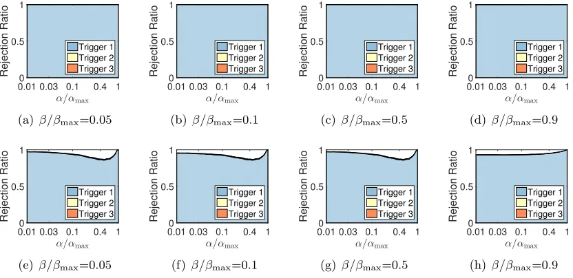
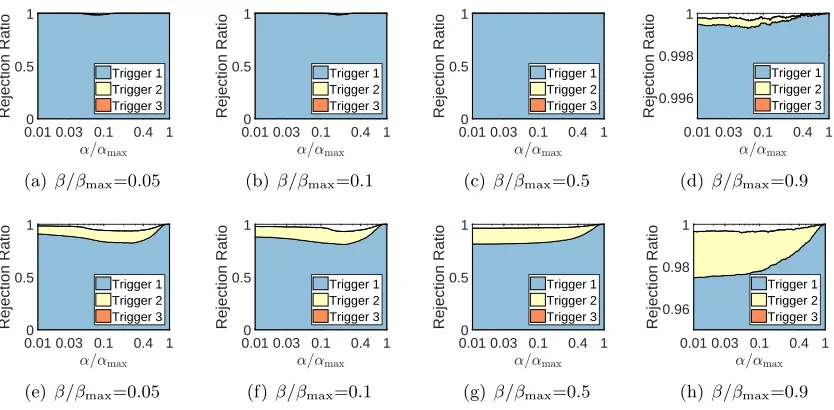
Due to the space limitation, we only report the rejection ratios of SIFS on syn2. Other results can be found in the appendix. Fig. 2 shows that SIFS can identify most of the inactive features and samples. However, few features and samples are identified in the second and later triggerings of ISS and IFS. The reason may be that the task here is so simple that one triggering is enough.

(18)

significant speedups, that is, up to 76.8 times. Taking syn2 for example, without SIFS, the solver takes more than two hours to solve problem (P∗) at 1,000 pairs of parameter values. However, combined with SIFS, the solver only needs less than three minutes for solving the same set of problems. From the theoretical analysis in Shalev-Shwartz and Zhang 2016 for AProx-SDCA, we can see that its computational complexity rises proportionately to the sample sizen and the feature dimensionp. From this theoretical result, we can see that the results in Fig. 1 are roughly consistent with the speedups we achieved shown in Table 1.

α/αmax 0.01 0.03 0.1 0.4 1

Rejection Ratio ₀

0.5 1

Trigger 1 Trigger 2 Trigger 3

(a)β/βmax=0.05

α/αmax 0.01 0.03 0.1 0.4 1

Rejection Ratio ₀

0.5 1

(b) β/βmax=0.1

α/αmax 0.01 0.03 0.1 0.4 1

Rejection Ratio ₀

0.5 1

(c)β/βmax=0.5

α/αmax 0.01 0.03 0.1 0.4 1

Rejection Ratio ₀

0.5 1

(d) β/βmax=0.9

α/α

max 0.01 0.03 0.1 0.4 1

Rejection Ratio ₀

0.5 1

(e)β/βmax=0.05

α/α

max 0.01 0.03 0.1 0.4 1

Rejection Ratio ₀

0.5 1

(f)β/βmax=0.1

α/α

max 0.01 0.03 0.1 0.4 1

Rejection Ratio ₀

0.5 1

(g)β/βmax=0.5

α/α

max 0.01 0.03 0.1 0.4 1

Rejection Ratio ₀

0.5 1

(h) β/βmax=0.9

Figure 2: Rejection ratios of SIFS on syn 2 (first row: Feature Screening, second row: Sample Screening).

Data Solver ISS+Solver IFS+Solver SIFS+Solver

ISS Solver Speedup IFS Solver Speedup SIFS Solver Speedup

syn1 499.1 4.9 27.8 15.3 2.3 42.6 11.1 8.6 6.0 34.2

syn2 8749.9 24.9 1496.6 5.8 23.0 288.1 28.1 92.6 70.3 53.7

syn3 1279.7 2.0 257.1 4.9 2.2 33.4 36.0 7.2 9.5 76.8

Table 1: Running time (in seconds) for solving problem (P∗) at 1,000 pairs of parameter values on three synthetic data sets.

6.2. Experiments with Sparse SVMs on Real Datasets

In this experiment, we evaluate the performance of SIFS on 5 large-scale real data sets: real-sim, rcv1-train, rcv1-test, url, and kddb, which are all collected from the project page of LibSVM (Chang and Lin, 2011). See Table 2 for a brief summary. We note that, the kddb data set has about 20 million samples with 30 million features.

(19)

they perform their method along with the training process and thus the size of the problem would keep decreasing during the iterations. Thus, comparing SIFS with this baseline in terms of the rejection ratios is inapplicable. We compare the performance of SIFS with the method in Shibagaki et al. 2016 in terms of speedup, i.e., the speedup gained by these two methods in solving problem (P∗) at 1,000 pairs of parameter values. The code of the method in Shibagaki et al. 2016 is obtained from (https://github.com/husk214/s3fs).

Dataset Feature size: p Sample size:n Classes

real-sim 20,958 72,309 2

rcv1-train 47,236 20,242 2

rcv1-test 47,236 677, 399 2

url 3,231,961 2,396,130 2

kddb 29,890,095 19,264,097 2

Table 2: Statistics of the binary real data sets.

0.01 0.03 0.1 0.4 1 0.97

0.98 0.99 1

Rejection Ratio

(a)β/βmax=0.05

0.01 0.03 0.10 0.4 1 0.5

1

Rejection Ratio

(b) β/βmax=0.1

0.01 0.03 0.10 0.4 1 0.5

1

Rejection Ratio

(c)β/βmax=0.5

0.01 0.03 0.10 0.4 1 0.5

1

Rejection Ratio

(d) β/βmax=0.9

0.01 0.03 0.10 0.4 1 0.5

1

Rejection Ratio

(e)β/βmax=0.05

0.01 0.03 0.10 0.4 1 0.5

1

Rejection Ratio

(f)β/βmax=0.1

0.01 0.03 0.1 0.4 1 0.9

0.95 1

Rejection Ratio

(g)β/βmax=0.5

0.01 0.03 0.1 0.4 1 0.985

0.99 0.995 1

Rejection Ratio

(h) β/βmax=0.9

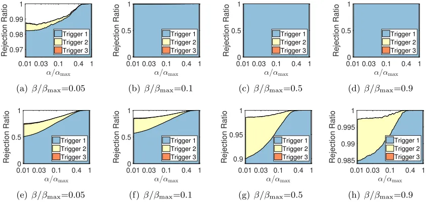
Figure 3: Rejection ratios of SIFS on real-sim when it performsISS first (first row: Feature Screening, second row: Sample Screening).

Fig. 3 shows the rejection ratios of SIFS on the real-sim data set (other results are in the appendix). In Fig. 3, we can see that some inactive features and samples are identified in the 2nd and 3rd triggerings of ISS and IFS, which verifies the necessity of the alternating application of ISS and IFS. SIFS is efficient since it always stops in 3 times of triggering. In addition, most of (>98%) the inactive features can be identified in the 1st triggering of IFS while identifying inactive samples needs to apply ISS two or more times. It may due to two reasons: 1) we run ISS first, which reinforces the capability of IFS due to the synergistic effect (see Sections 4.1 and 4.2), referring to the analysis below for further verification; 2) feature screening here may be easier than sample screening.

(20)

sets. The speedup gained by SIFS is up to 300 times on real-sim, rcv1-train and rcv1-test. Moreover, SIFS significantly outperforms the method in Shibagaki et al. 2016 in terms of speedup—by about 30 to 40 times faster on the aforementioned three data sets. For data sets url and kddb, we do not report the results of the solver as the sizes of the data sets are huge and the computational cost is prohibitive. Instead, we can see that the solver with SIFS is about 25 times faster than the solver with the method in Shibagaki et al. 2016 on both data sets url and kddb. Let us take the data set kddb as an example. The solver with SIFS takes about 13 hours to solve problem (P∗) for 1,000 pairs of parameter values, while the solver with the method in Shibagaki et al. 2016 needs 11 days to finish the same task.

Data

Set Solver

Method in Shibagaki et al. 2016+Solver SIFS+Solver

Screen Solver Speedup Screen Solver Speedup

real-sim 3.93E+04 24.10 4.94E+03 7.91 60.01 140.25 195.00

rcv1-train 2.98E+04 10.00 3.73E+03 7.90 27.11 80.11 277.10

rcv1-test 1.10E+06 398.00 1.35E+05 8.10 1.17E+03 2.55E+03 295.11

url >3.50E+06 3.18E+04 8.60E+05 >4.00 7.66E+03 2.91E+04 >100

kddb >5.00E+06 4.31E+04 1.16E+06 >4.00 1.10E+04 3.6E+04 >100

Table 3: Running time (in seconds) for solving problem (P∗) at 1,000 pairs of parameter values on five real data sets.

0.01 0.03 0.1 0.4 1 0.97

0.98 0.99 1

Rejection Ratio

(a)β/βmax=0.05

0.01 0.03 0.10 0.4 1 0.5

1

Rejection Ratio

(b) β/βmax=0.1

0.01 0.03 0.10 0.4 1 0.5

1

Rejection Ratio

(c)β/βmax=0.5

0.01 0.03 0.10 0.4 1 0.5

1

Rejection Ratio

(d) β/βmax=0.9

0.01 0.03 0.10 0.4 1 0.5

1

Rejection Ratio

(e)β/βmax=0.05

0.01 0.03 0.10 0.4 1 0.5

1

Rejection Ratio

(f)β/βmax=0.1

0.01 0.03 0.1 0.4 1 0.9

0.95 1

Rejection Ratio

(g)β/βmax=0.5

0.01 0.03 0.1 0.4 1 0.985

0.99 0.995 1

Rejection Ratio

(h) β/βmax=0.9

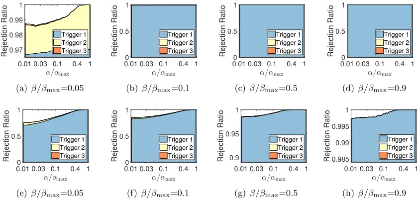
Figure 4: Rejection ratios of SIFS on real-sim when it performsIFS first(first row: Feature Screening, second row: Sample Screening).

(21)

first are also much higher than those in Fig. 3(e)-3(h) where SIFS performs ISS first. This demonstrates that the screening result of ISS can reinforce the capability of IFS and vice versa, which is the so called synergistic effect. At last, in Fig. 4 and Fig. 3, we can see that the overall rejection ratios at the end of SIFS are exactly the same. Hence, no matter which rule (ISS or IFS) we perform first in SIFS, SIFS has the same screening performances in the end, which verifies the conclusion we present in Theorem 12.

Performance in Solving Single ProblemsIn the experiments above, we solve prob-lem (P∗) at a grid of turning parameter values. This setting is meaningful and it arises naturally in various cases, such as cross validation (Kohavi, 1995) and feature selection (Meinshausen and B¨uhlmann, 2010; Yang et al., 2015). Therefore, the results above demon-strate that our method would be helpful in such real applications. We notice that sometimes one may be interested in the model at a specific parameter value pair. To this end, we now evaluate the performance of our method in solving a single problem. Due to the space limitation, we solve sparse SVM at 16 specific parameter values pairs on the real-sim data set for examples, To be precise, β∈ {0.05,0.10,0.5,0.9} and each β has 4 values of α satisfying

α/αmax(β) ∈ {0.05,0.1,0.5,0.9}. For each (αi, βi), we construct a parameter value path {(αj,i, βi), j = 0, ..., M} with αj,i equally spaced at the logarithmic scale of αj,i/αmax(βi)

between 1 and αi/αmax(βi), which implies that αmax(βi) = α0,i > α1,i > ... > αM,i =αi.

Then we use AProx-SDCA integrated with SIFS to solve problem (P∗) at the parameter value pairs on the path one by one and report the total time cost. It can be expected that for

αi far from αmax(βi), we need more points on the parameter value path in order to obtain

higher rejection ratios and more significant speedups of SIFS and otherwise we need fewer ones. In this experiment, we fixM = 50 at each αi for convenience. For comparison, we

solve the problem at (αi, βi) using AProx-SDCA with random initializations, which would be

faster than solving all the problems on the path. Table 4 reports the speedups achieved by SIFS at these parameter value pairs. It shows that SIFS can still obtain significant speedups. In addition, compared with the results in Tables 1 and 3, we can see that our method is much better at solving a problem sequence than solving a single problem.

XX XX

XX

XX_X

β/βmax

α/αmax(β)

0.05 0.10 0.50 0.90

0.05 6.31 7.14 21.04 146.66 0.10 6.14 7.18 21.83 156.63 0.50 5.75 7.18 20.99 154.60 0.90 6.39 7.66 23.16 173.56

Table 4: The speedups achieved by SIFS in solving single problems

6.3. Experiments with Multi-class Sparse SVMs

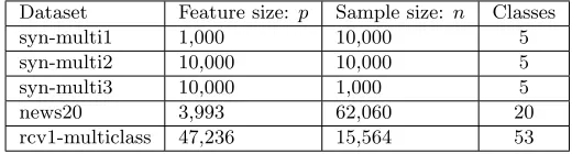
We evaluate SIFS for multi-class Sparse SVMs on 3 synthetic data sets (multi1, syn-multi2, and syn-multi3) and 2 real data sets (news20 and rcv1-multiclass). Their statistics are given in Table 5.

The synthetic data sets are generated in a similar way as we did in Section 6.1. Each of them has K = 5 classes and each class has n/K samples. The data points of them can be written as x = [x1;x2], where x1 = [x1₁;...;xK₁ ] ∈ R0.02p with xk1 ∈ R0.02p/Kand x2 ∈_R0.98p_{. If}_x _{belongs to the}_k_{-th class, then} _xk

(22)

G = N(u,0.75I) with u = 1.51, I ∈ _R(0.02p/K)×(0.02p/K) _{and other components in} _x 1 are from N(0,1). Each entry of x2 has chanceη = 0.2 to be sampled from distributionN(0,1) and chance 1−η to be 0.

Dataset Feature size:p Sample size: n Classes

syn-multi1 1,000 10,000 5

syn-multi2 10,000 10,000 5

syn-multi3 10,000 1,000 5

news20 3,993 62,060 20

rcv1-multiclass 47,236 15,564 53

Table 5: Statistics of the multi-class data sets.

Fig. 5 shows the scaling ratios of ISS, IFS, and SIFS on the synthetic data sets at 1,000 pairs of parameter values. Similar to the results in sparse SVMs, SIFS totally surpasses IFS and ISS, with scaling ratios larger than 98% at any parameter value pair against 70−90%. Thus, we can expect significant speedups by integrating SIFS with the solver.

-2 -1.5 -1 -0.5 0

log( / _max)

0 -0.7 -1 -1.3

log(

/ max

)

-2 -1.5 -1 -0.5 0

log( / _max)

0 -0.7 -1 -1.3

-2 -1.5 -1 -0.5 0

log( / _max)

0 -0.7 -1 -1.3

0.95 1

(a) syn-multi1.

-2 -1.5 -1 -0.5 0

log( /

max)

0 -0.7 -1 -1.3

log(

/ max

)

-2 -1.5 -1 -0.5 0

log( /

max)

0 -0.7 -1 -1.3

-2 -1.5 -1 -0.5 0

log( /

max)

0 -0.7 -1 -1.3

0.8 0.9 1

(b) syn-multi2.

-2 -1.5 -1 -0.5 0

log( /

max)

0 -0.7 -1 -1.3

log(

/ max

)

-2 -1.5 -1 -0.5 0

log( /

max)

0 -0.7 -1 -1.3

-2 -1.5 -1 -0.5 0

log( /

max)

0 -0.7 -1

-1.3 0.7

0.8 0.9

(c) syn-multi3.

Figure 5: Scaling ratios of ISS, IFS, and SIFS (from left to right).

Fig. 6 and 7 present the rejection ratios of SIFS on the news20 data set (the results of other data sets can be found in the appendix). It indicates that, by alternatively applying IFS and ISS, we can finally identify most of the inactive samples (> 95%) and features (>99%). The synergistic effect between IFS and ISS can also be found in these figures.

(23)

0.01 0.03 0.10 0.4 1 0.5 1 Rejection Ratio Trigger 1 Trigger 2 Trigger 3

(a)β/βmax=0.05

0.01 0.03 0.10 0.4 1

0.5 1 Rejection Ratio Trigger 1 Trigger 2 Trigger 3

(b) β/βmax=0.1

0.01 0.03 0.10 0.4 1

(c)β/βmax=0.5

0.01 0.03 0.1 0.4 1

0.996 0.998 1 Rejection Ratio Trigger 1 Trigger 2 Trigger 3

(d) β/βmax=0.9

0.01 0.03 0.10 0.4 1

(e)β/βmax=0.05

0.01 0.03 0.10 0.4 1

(f)β/βmax=0.1

0.01 0.03 0.10 0.4 1

(g)β/βmax=0.5

0.01 0.03 0.1 0.4 1

(h) β/βmax=0.9

Figure 6: Rejection ratios of SIFS on syn-multi2 (first row: Feature Screening, second row: Sample Screening).

0.03 0.1 0.4 1

(a)β/βmax=0.05

0.03 0.1 0.4 1

(b) β/βmax=0.1

0.01 0.03 0.10 0.4 1

(c)β/βmax=0.5

0.01 0.03 0.10 0.4 1

(d) β/βmax=0.9

0.03 0.1 0.4 1

(e)β/βmax=0.05

0.03 0.1 0.4 1

(f)β/βmax=0.1

0.01 0.03 0.10 0.4 1

(g)β/βmax=0.5

0.01 0.03 0.10 0.4 1

(h) β/βmax=0.9

Figure 7: Rejection ratios of SIFS on news20 (first row: Feature Screening, second row: Sample Screening).

(24)

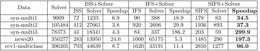
SIFS and IFS on syn-multi3 is far greater than those gained on syn-multi1 and syn-multi2. The reason is that the convergence rate of the solver in our problem may depend on the condition number of the data matrix. The dimension of w in syn-multi3 is much larger than its sample size (50,000 over 1,000), which leads to a large condition number and a bad convergence rate. However, SIFS and IFS can remove the inactive features from the model, which can greatly improve the convergence rate of the solver by decreasing the condition number. This point can also be supported by the fact in the experiment on syn-multi3 that the solver with SIFS or IFS needs much fewer iterations to converge to the optima than that without SIFS or IFS.

Data Solver ISS+Solver IFS+Solver SIFS+Solver

ISS Solver Speedup IFS Solver Speedup SIFS Solver Speedup

syn-multi1 9009 72 1233 6.9 90 388 18.9 178 83 34.5

syn-multi2 105484 412 27661 3.8 920 2606 29.9 1936 893 37.3

syn-multi3 78373 44 18341 4.3 84 337 186.2 203 59 299.9

news20 350277 283 13950 24.6 1000 65175 5.3 1485 290 197.3

rcv1-multiclass 396205 793 44639 8.7 1620 33191 11.4 2850 1277 96.0

Table 6: Running time (in seconds) for solving problem (m-P∗) at 1,000 pairs of parameter values on synthetic and real data sets.

7. Conclusions

In this paper, we proposed a novel data reduction method SIFS to simultaneously identify inactive features and samples for sparse SVMs. Our major contribution is a novel framework for an accurate estimation of the primal and dual optima based on strong convexity. To the best of our knowledge, the proposed SIFS is the first static screening method that is able to simultaneously identify inactive features and samples for sparse SVMs. An appealing feature of SIFS is that all detected features and samples are guaranteed to be irrelevant to the outputs. Thus, the model learned on the reduced data is exactly identical to that learned on the full data. To show the flexibility of the proposed SIFS, we extended it to multi-class sparse SVMs. The experimental results demonstrate that, for both sparse SVMs and multi-class sparse SVMs, SIFS can dramatically reduce the problem size and the resulting speedup can be orders of magnitude. We plan to generalize SIFS to more complicated models, e.g., SVMs with a structured sparsity-inducing penalty.

Acknowledgments

(25)

Appendix A. Detailed Proofs and More Experimental Results

In this appendix, we first present the detailed proofs of all the theorems in the main paper and then report the rest experimental results which are omitted in the experimental section.

A.1. Proof for Lemma 3 Proof of Lemma 3:

1) It is the immediate conclusion of the analysis above.

2) After feature screening, the primal problem (P∗) is scaled into:

min ˜

w∈R|Fˆc| α

2||w˜||

2₊_β_||_w_˜_|| 1+

1

n n X

i=1

`(1− h[¯xi]_Fˆc,w˜i). (scaled-P∗-1)

Thus, we can easily derive out the dual problem of (scaled-P∗-1):

min ˜

θ∈[0,α]n

˜

D(˜θ;α, β) = 1 2α||Sβ(

1

nFˆc[ ¯X]˜θ)||

2₊ γ 2n||

˜

θ||2₋ 1

nh1,

˜

θi, (scaled-D∗-1)

and the KKT conditions:

˜

w∗(α, β) = 1

αSβ(

1

nFˆc[ ¯X]˜θ

∗₍_{α, β}₎₎_, _{(scaled-KKT-1)}

[˜θ∗(α, β)]_i =







0, if 1− h[¯xi]Fˆc,w˜∗(α, β)i<0,

1

γ(1− h[¯xi]Fˆc,w˜∗(α, β)), if 0≤1− h[¯xi]_Fˆc,w˜∗(α, β)≤γ,

1, if 1− h[¯xi]Fˆc,w˜∗(α, β)> γ,

(scaled-KKT-2)

Then, it is obvious that ˜w∗(α, β) = [w∗(α, β)]Fˆc, since essentially, problem (scaled-P∗-1)

can be derived by substituting 0 to the weights for the eliminated features in problem (P∗) and optimizing over the rest weights.

Since the solutions w∗(α, β) andθ∗(α, β) satisfy the conditions (KKT-1) and (KKT-2) and

h[¯xi]Fˆc,w˜∗(α, β)i=hx¯i,w∗(α, β)i for alli, we know that ˜w∗(α, β) andθ∗(α, β) satisfy the

conditions (scaled-KKT-1) and (scaled-KKT-2). Thus they are the solutions of problems (scaled-P∗-1) and (scaled-D∗-1). Then, due to the uniqueness of the solution of problem (scaled-D∗-1), we have

θ∗(α, β) = ˜θ∗(α, β). (27)

From 1) we have [˜θ∗(α, β)]Rˆc = 0 and [˜θ∗(α, β)]Lˆc = 1. Therefore, from the dual problem

(scaled-D∗), we can see that [˜θ∗(C, α)]Dˆc can be recovered from the following problem:

min ˆ

θ∈[0,1]|Dˆ

c|

1 2α||Sβ(

1

n

ˆ G1θˆ+ 1

n

ˆ

G21)||2+ γ 2n||

ˆ

θ||2− 1 nh1,

ˆ

θi.

(26)

(i) We prove this lemma by verifying that the solutions w∗(α, β) =0 andθ∗(α, β) =1 satisfy the conditions (KKT-1) and (KKT-2).

Firstly, since β ≥βmax = ||_n1X1¯ ||∞, we have Sβ(_n1X1¯ ) = 0. Thus w∗(α, β) = 0 and θ∗(α, β) =1 satisfy the condition (KKT-1).

Then, for alli∈[n], we have

1− hx¯i,w∗(α, β)i= 1−0> γ.

Thus, w∗(α, β) =0 and θ∗(α, β) = 1 satisfy the condition (KKT-2). Hence, they are the solutions of the primal problem (P∗) and the dual problem (D∗), respectively.

(ii) Similar to the proof of (i), we prove this by verifying that the solutions w∗(α, β) = 1

αSβ(

1

nX¯θ

∗₍_{α, β}_{)) and}_θ∗₍_{α, β}_{) =}₁ _{satisfy the conditions (KKT-1) and (KKT-2).}

1. Case 1: αmax(β)≤0. Then for all α >0, we have min

i∈[n]

{1− hx¯i,w∗(α, β)i}

= min

i∈[n]

{1− 1

αhx¯i,Sβ(

1

n

¯

Xθ∗(α, β))i}= min

i∈[n]

{1− 1

αhx¯i,Sβ(

1

n

¯ X1)i}

=1− 1 αmax_i∈[n]

hx¯i,Sβ(

1

nX1¯ )i= 1−(1−γ)

1

ααmax(β) ≥1> γ.

Then, L= [n], andw∗(α, β) = _α1S_β(_n1X¯θ∗(α, β)) and θ∗(α, β) =1 satisfy the condi-tions (KKT-1) and (KKT-2). Hence, they are the optimal solution of the primal and dual problems (P∗) and (D∗).

2. Case 2: αmax(β)>0. Then for any α≥αmax(β), we have min

i∈[n]

{1− hx¯i,w∗(α, β)i}

= min

i∈[n]

{1− 1

αh¯xi,Sβ(

1

nX¯θ

∗₍_{α, β}₎₎_i}_{= min}

i∈[n]

{1− 1

αhx¯i,Sβ(

1

nX1¯ )i}

=1− 1 αmaxi∈[n]

hx¯i,Sβ(

1

n

¯

X1)i= 1−(1−γ)1

ααmax(β)≥1−(1−γ) =γ.

Thus, E ∪ L = [n], and w∗(α, β) = _α1Sβ(1_nX¯θ∗(α, β)) and θ∗(α, β) = 1 satisfy the

conditions (KKT-1) and (KKT-2). Hence, they are the optimal solution of the primal and dual problems (P∗) and (D∗).

(27)

Due to the α-strong convexity of the objective P(w;α, β), we have

P(w∗(α0, β0);α, β0)≥P(w∗(α, β0);α, β0) +

α

2||w ∗

(α0, β0)−w∗(α, β0)||2,

P(w∗(α, β0);α0, β0)≥P(w∗(α0, β0);α0, β0) +

α0 2 ||w

∗₍_α

0, β0)−w∗(α, β0)||2, which are equivalent to

α

2||w ∗₍_α

0, β0)||2+β0||w∗(α0, β0)||1+L(w∗(α0, β0))

≥ α

2||w ∗₍_{α, β}

0)||2+β0||w∗(α, β0)||1+L(w∗(α, β0)) +

α

2||w ∗₍_α

0, β0)−w∗(α, β0)||2,

α0 2 ||w

∗

(α, β0)||2+β0||w∗(α, β0)||1+L(w∗(α, β0))

≥ α0

2 ||w ∗

(α0, β0)||2+β0||w∗(α0, β0)||1+L(w∗(α0, β0)) +

α0 2 ||w

∗

(α0, β0)−w∗(α, β0)||2. Adding the above two inequalities together, we obtain

α−α0 2 ||w

∗₍_α

0, β0)||2≥

α−α0 2 ||w

∗₍_{α, β}

0)||2+

α0+α

2 ||w ∗₍_α

0, β0)−w∗(α, β0)||2

⇒ ||w∗(α, β0)−

α0+α

2α w

∗₍_α

0, β0)||2 ≤

(α−α0)2 4α2 ||w

∗₍_α

0, β0)||2. (28) Substituting the prior that [w∗(α, β0)]_Fˆ = 0 into Eq. (28), we obtain

||[w∗(α, β0)]Fˆc−

α0+α

2α [w

∗₍_α

0, β0)]Fˆc||2 ≤(α−α0)

2 4α2 ||w

∗

(α0, β0)||2−

(α0+α)2 4α2 ||[w

∗

(α0, β0)]Fˆ|| 2_. The proof is complete.

A.4. Proof for Lemma 6

Proof of Lemma 6: Firstly, we need to extend the definition ofD(θ;α, β) to Rn:

˜

D(θ;α, β) =

D(θ;α, β), ifθ∈[0,1]n,

+∞, otherwise. (29)

Due to the strong convexity of objective ˜D(θ;α, β), we have

˜

D(θ∗(α0, β0), α, β0)≥D˜(θ∗(α, β0), α, β0) +

γ

2n||θ

∗₍_α

0, β0)−θ∗(α, β0)||2, ˜

D(θ∗(α, β0), α0, β0)≥D˜(θ∗(α0, β0), α0, β0) +

γ

2n||θ

∗