Policy Optimization with Model-Based Explorations

The Thirty-Third AAAI Conference on Artificial Intelligence (AAAI-19)

Policy Optimization with Model-Based Explorations

Feiyang Pan,

_{Qingpeng Cai,}

_{An-Xiang Zeng,}

_{Chun-Xiang Pan,}

_{Qing Da,}

Hualin He,

_{Qing He,}

_{Pingzhong Tang}

1_{Key Lab of Intelligent Information Processing of Chinese Academy of Sciences (CAS),}

Institute of Computing Technology, CAS, Beijing 100190, China.{panfeiyang, heqing}@ict.ac.cn

2_{University of Chinese Academy of Sciences, Beijing 100049, China.} 3_{IIIS, Tsinghua University. [email protected], [email protected]} 4_{Alibaba Group.{renzhong, xuanran}@taobao.com,{daqing.dq, hualin.hhl}@alibaba-inc.com}

Abstract

Model-free reinforcement learning methods such as the Prox-imal Policy Optimization algorithm (PPO) have successfully applied in complex decision-making problems such as Atari games. However, these methods suffer from high variances and high sample complexity. On the other hand, model-based reinforcement learning methods that learn the transition dy-namics are more sample efficient, but they often suffer from the bias of the transition estimation. How to make use of both model-based and model-free learning is a central problem in reinforcement learning.

In this paper, we present a new technique to address the trade-off between exploration and exploitation, which regards the difference between model-free and model-based estimations as a measure of exploration value. We apply this new tech-nique to the PPO algorithm and arrive at a new policy op-timization method, named Policy Opop-timization with Model-based Explorations (POME). POME uses two components to predict the actions’ target values: a model-free one es-timated by Monte-Carlo sampling and a model-based one which learns a transition model and predicts the value of the next state. POME adds the error of these two target estima-tions as the additional exploration value for each state-action pair, i.e, encourages the algorithm to explore the states with larger target errors which are hard to estimate. We compare POME with PPO on Atari 2600 games, and it shows that POME outperforms PPO on 33 games out of 49 games.

Introduction

Reinforcement Learning focuses on maximizing long-term return by interacting with the environment sequentially (Sut-ton and Barto 1998). Generally, a reinforcement learning al-gorithm has two aspects, on the one hand, it estimates the

∗

These authors contributed equally in this work. †

The research was supported by the National Key Re-search and Development Program of China under Grant No. 2017YFB1002104, the National Natural Science Foundation of China under Grant No. 61602438, 91546122, 61573335, Guang-dong provincial science and technology plan projects under Grant No. 2015 B010109005.

‡

Pingzhong Tang and Qingpeng Cai were supported in part by the National Natural Science Foundation of China Grant 61561146398, a China Youth 1000-talent program and an Alibaba Innovative Research program.

Copyright c2019, Association for the Advancement of Artificial Intelligence (www.aaai.org). All rights reserved.

state-action value function (also known as the Q-function), on the other hand, it optimizes or improves the policy to maximize its performance measure.

There are two classes of reinforcement learning methods, model-free and model-based methods. Model-free methods (Peters and Schaal 2006) estimate and iteratively update the state-action value with the rollout samples by Temporal Dif-ference learning (Sutton and Barto 1998). It is said that model-based methods maintain an approximate model in-cluding the reward functions and the state transitions, and then use the approximated rewards and transitions to es-timate the value function. Model-based methods are more efficient than model-free methods (Li and Todorov 2004; Levine and Koltun 2013; Montgomery and Levine 2016; Wahlstr¨om, Sch¨on, and Desienroth 2015; Watter et al. 2015) especially in discrete environments by reducing the sample complexity. Model-free methods are more generally appli-cable to continuous and complex control problems but may suffer from high sample complexity (Schulman et al. 2015; Lillicrap et al. 2015).

Model-free methods directly use the immediate rewards and next states from rollout samples and estimate the long-term state-action value by Temporal Difference learning, for example, Sarsa or Q-learning (Sutton and Barto 1998). Therefore, the target value is unbiased but may induce large variance due to the randomness of the transition dynam-ics or the off-policy stochastic exploration strategy. Model-based methods use the prediction of the immediate reward and the next state by its own belief of the environment. The belief of the agent, including the approximate reward func-tion and transifunc-tion model, is updated after receiving more signals from the environment. So the estimated target value in model-based methods is often biased due to the approx-imation error of the model, but it has low variance com-pared with model-free methods. Combining model-based and model-free learning has been an important question in the recent literature.

We aim to answer the following question: How to incor-porate model-based and model-free methods for better con-trol?

transition model to supplement the real transition samples. (Cai, Pan, and Tang 2018) uses a convex combination of the two target values as the new target, following the insight that the ensemble could more accurate. But the large loss of model prediction would also lead to an incorrect update for policy iteration.

In this paper, we incorporate the two methods together to address the trade-off between exploration and exploita-tion (EE), by a simple heuristic that adds the discrepancy between both target values as a relative measure of the ex-ploration value, so as to encourage the agent to explore more difficult transition dynamics.

The trade-off between EE is a fundamental and challeng-ing problem in reinforcement learnchalleng-ing because it is hard to evaluate the value of exploring unfamiliar states and ac-tions. Model-free exploration methods are widely discussed over decades. To name some, Upper Confidence Bounds (Auer, Cesa-Bianchi, and Fischer 2002; Li et al. 2010; Chen et al. 2017) adds the upper confidence bound of the uncertainty of value estimation as an exploration value of actions. Thompson Sampling (Thompson 1933) can also be understood as adding stochastic exploration value based on the posterior distribution of value estimation (May et al. 2012). However these model-free value-based methods of-ten require a table to store the number of visits of each state-action pair so that the uncertainty of value estimation can be delivered (Tang et al. 2017), so they are not practical to handle problems with continuous state spaces such as Atari games or large-scale real-world problems such as mecha-nism design (Tang 2017) and e-commerce (Cai et al. 2018a; 2018b). Model-based methods for deep RL can have bet-ter exploration based on maximization of information gain (Houthooft et al. 2016) or minimization of error (Pathak et al. 2017) about the agents’ belief, however, may be unstable due to the difficulty of learning the transition dynamics.

In this paper, based on the discrepancy between model-free and model-based target values, we present a new al-gorithm named Policy Optimization with Model-based Ex-ploration (POME), an exploratory modified version of the well-known algorithm Proximal Policy Optimization (PPO). Different from previous methods, we use the model-free sample-based estimator for the advantage function as the base for POME, which is already successfully used in var-ious actor-critic methods including PPO. Then POME adds a centralized and clipped exploration bonus onto the advan-tage value, so as to encourage exploration as well as stabilize the performance.

Our intuition is that the discrepancy of target values of model-based and model-free methods can be understood as the uncertainty of the transition dynamics. A high explo-ration value means that the transition of the state-action pair is hard to estimate and needs to be explored. We directly add the difference to the advantage estimation as the exploration bonus of the state-action pair. So if the exploration value of a state-action pair is higher than average, POME will encour-age the encour-agent to visit it more frequently in the future so as to better learn the transition dynamics. If not, POME will reduce the chance of picking it and give the agent an oppor-tunity to try other actions.

We verify POME on the Atari 2600 game playing bench-marks. We compare our POME with the original model-free PPO algorithm and a model-based extended version of PPO. Experimental results show that POME outperforms the orig-inal PPO on 33 Atari games out of 49. We also tested two versions of POME, one with decaying exploration level and the other with non-decaying exploration level, which results in an interesting finding that the exploration bonus can im-prove the performance even in a long run.

Background and Notations

A Markov Decision Process (MDP) is defined as the tuple

(S,A, r, P, P0), whereSis the (discrete or continuous) state space, A is the (discrete or continuous) action space, r :

S × A → _Ris the (immediate) reward function,P is the state transition model, andP0is the probability distribution for the initial states0.

The goal of the agent is to find the policyπ∗ from a re-stricted family of parametrized policy functions that maxi-mizes its performance,

π∗= arg max

π∈ΠJ(π), (1)

whereJ(π)is the performance objective defined as

J(π) =_Es0,a0,s1,...

∞

X

t=0

γtr(st, at)|π, s0∼P0

, (2)

whereγ∈(0,1)is a discount factor that balances the short-and long-term returns. For convenience, letρπ_{(s)denote the} (unnormalized) discounted cumulated state distribution in-duced by policyπ,

ρπ(s) :=

∞ X

t=0

γtPr(st=s|π, s0∼P0) (3)

then the performance objective can rewrite as

J(π) =_Es∼ρπ_,a∼π[r(s, a)].

Since the expected long-term return is unknown, the basic idea behind RL is to construct a tractable estimator to ap-proximate the actual return. Then we can update the policy in the direction that the performance measure is guaranteed to improve at every step (Kakade and Langford 2002). Let Qπ_{(s, a)denote the expected action value of actionaat state} sby following policyπ, i.e.

Qπ(s, a) =E

∞

X

t=0

γtr(st, at)|s0=s, a0=a, π

. (4)

And we write the state valueVπ(s)and the advantage action valueAπ_{(s, a)as}

Vπ(s) =

Z

A

π(a|s)Qπ(s, a)da, (5)

Aπ(s, a) =Qπ(s, a)−Vπ(s). (6)

Since we have the Bellman equation

Qπ(s, a) =r(s, a) +γEs0[Vπ(s0)], (7) the advantage function can also be written as

Aπ(s, a) =r(s, a) +γ_Es0[Vπ(s0)]−Vπ(s). (8) In practice, estimations of these quantities are used to evaluate the policy and to guide the direction of policy up-dates.

Policy Optimization Methods

Policy Gradient (PG) methods (Sutton et al. 2000) compute the gradient ofJ(πθ)w.r.t policy parametersθand then use gradient ascent to update the policy. The well-known form of policy gradient writes as follow

∇θJ(πθ) =Es∼ρπθ,a∼πθ

Aπθ_{(s, a)∇}

θlogπθ(a|s)

. (9)

Instead of directly using the policy gradients, trust region based methods use a surrogate objective to perform policy optimization. For the reason that the trajectory distribution is known only for the prior policyπold before the update,

trust region based methods introduce the following local ap-proximation toJ(πθ)for any untested policyπθ, as

Lπold(πθ) =J(πold) +Es∼ρπold,a∼πθ[πθ(a|s)A

πold_{(s, a)].}

(10) It is proved (Kakade and Langford 2002; Schulman et al. 2015) that if the new policy πθ is close to the πold in the

sense of the KL divergence, there is a lower bound of the long-term rewards of the new policy. For the general case, we have the following result:

Theorem 1 (Schulman et al. 2015). Let

Dmax

KL (πold, πθ) = maxsKL[πold(·|s)kπθ(·|s)] and Amax= maxs|Ea∼πθ[A

πold_{(s, a)]|. The performance of the}

policyπ˜can be bounded by

J(πθ)≥Lπold(πθ)−

2γAmax

(1−γ)2D max

KL (πold, πθ). (11)

By following Theorem 1, there is a category of policy it-eration algorithms with monotonic improvement guarantee, known as conservative policy iteration (Kakade and Lang-ford 2002). Among them, Trust Region Policy Optimization (TRPO) is one of the most widely used baselines to optimize parametric policies to solve complex or continuous prob-lems. The optimization problem w.r.t the new parameterθ is

max

θ Es∼ρ

π_old,a∼π

old

_π

θ(a|s) πold(a|s)A

πold_{(s, a)}

(12)

s.t. KL[πold(·|s)kπθ(·|s)]≤δKLfor alls.

whereδKL is a hard constraint for the KL-divergence. In practice, the hard constraint of KL-divergence is softened by an expectation over visited states and moved to the objective with a multiplierβso that it becomes an unconstrained op-timization problem, i.e.

max

θ E

πθ(a|s) πold(a|s)

Aπold_{(s, a)−βKL[πold(·|s)kπ}

θ(·|s)]

,

(13)

which stabilise standard RL objectives.

Proximal Policy Optimization (PPO) (Schulman et al. 2017) can be view as a modified version of TRPO, which mainly uses a clipped probability ratio in the objective to avoid excessively large policy updates. It mainly replaces the term inside the expectation in (12) with

lPPO(θ;s,a) = minπθ(a|s) πold(a|s)

Aπold_{(s, a),}

clip πθ(a|s)

πold(a|s),1−,1 +

Aπold_{(s, a) .}

(14)

PPO is said to be empirically more sample efficient than TRPO, and is made one of the most frequently used base-lines in various kinds of deep RL tasks.

Policy Evaluation with Function Approximation

In the previous part, we show several objectives for policy optimization. The objectives commonly need to compute an expectation over(s, a)pairs obtained by following the cur-rent policy and an estimator of advantage values.

In on-policy methods such as TRPO and PPO, the expec-tation is approximated with the empirical average over sam-ples induced by the current policyπold. Therefore the policy

updates in a similar manner to the stochastic gradient de-scent as in modern supervised learning.

Model-free value estimation Model-free methods esti-mate the value functions by the samples in the rollout trajec-tory (s0, a0, r0, s1, . . . ,). By following the Bellman equa-tion, we can estimate the action or advantage value by Tem-poral Difference learning. When referring to the quantities at time steptof a trajectory, we will useQt,Vt, andAtfor short to denoteQ(st, at),V(at), andA(st, at)respectively. Policy-based methods, as described in the previous part, typically need to use the advantage valueAt. It is discussed in (Schulman et al. 2015; Wang et al. 2016) that it can be one of the following estimators without introducing bias: the state-action valueQt, the discounted return of the trajectory started from(st, at), the one-step temporal difference error (TD error)

δt=rt+γVt+1−Vt, (15)

or the k-step cumulated temporal difference error as used in the actual algorithm of PPO

δ_tk:=

k−1 X

j≥0

(γλ)jδt+j, (16)

whereλ is a discount coefficient to balance future errors. Whenλ = 1, the estimator naturally becomes the advan-tage approximation in the asynchronous advanadvan-tage actor critic algorithm (A3C) (Mnih et al. 2016)AA3C(st, at) =

Pk−1

j≥0γ j_r

t+j+γkVt+k−Vt. It is known that these estima-tors would not introduce bias to the policy gradient, but they have different variances.

to compute the temporal difference errors, the state value Vπ_{(s)is always approximated with a neural networkV}

φ(s), whereφis the network parameter. Then if the one-step TD error is computed with on-policy samples, it becomes a loss function w.r.t the parametersφ,

δt(φ) =Q∗f,t−Vφ(st), (17)

whereQ∗_f,tdenotes the model-free target value

Q∗_f,t=rt+γVφ(st+1). (18)

Therefore in many algorithms the value parameters are up-dated by minimizing the error on samples using stochastic gradient descent.

The methods discussed so far can be categorized into model-free methods, because the immediate rewards and the state transitions are sampled from the trajectories.

Model-based value estimation For the model-based case, additional function approximation should be used to esti-mate the reward function and the transition function, i.e.

ˆ

r(st, at)≈rt and Tˆ(st, at)≈st+1. (19)

In continuous problems the form ofrˆ(st, at)andTˆ(st, at) can be neural networks, which are trained by minimizing some error measures between the model predictions and the realrtandst+1. Here the symbols for parameters are omit-ted for simplicity. When using the mean squared error, we can define the loss function to these two networks

Lr=Ert−rˆ(st, at)

2

,LT =Ekst+1−Tˆ(st, at)k22 which can be minimized using stochastic gradient descent w.r.t the network parameters. To make use of the model-based estimators, similar to the model-free case, we have the model-based TD error

˜

δt(φ) =Q∗b,t−Vφ(st) (20)

as an alternative toδtin (17), whereQ∗b,tdenotes the

model-based target value

Q∗_b,t = ˆr(st, at) +γVφ( ˆT(st, at)). (21)

To solve complex tasks with high-dimensional inputs, model-free deep RL methods can often learn faster com-paring to model-based methods especially in the beginning, mainly because it has fewer parameters to learn.

Policy Optimization with Model-based

Explorations

In this section, we propose an extension of the trust re-gion based policy optimization method with the exploration heuristics by making use of the difference between the model-free and model-based value estimations.

Let us think of the TD error as a subtract between the tar-get value and the current function approximation. The tartar-get value for model-free and model-based learning is written in (18) and (21). Here we define thediscrepancy of targetsof state-action pair(st, at)as

t=|Q∗b,t−Q ∗

f,t| (22)

=|rt+γV(st+1)−rˆ(st, at)−γV( ˆT(st, at))|. (23)

For our method, we use this error as an additional explo-ration value for the pair (st, at). The proposed methods is named Policy Optimization with Model-based Exploration (POME). So the resulted TD error used in POME is

δPOME_t =δt+α(t−¯), (24)

whereα >0is a coefficient decaying to0and¯is used to shift the exploration bonus to zero mean over samples from the same batch.

Insights

The basic idea behind POME is to add an exploration bonus to the state-action pairs where there is a discrepancy between the model-based and model-free Q-values.

The intuition is that the discrepancy between both Q-values would be small if the agent is “familiar” with the transition dynamics, for example, when the probability dis-tribution of the next state concentrates on one deterministic state and at the meanwhile the next state has already been visited several times. On another hand, the error would be large if the agent is uncertain about what is going on, for example, if it has trouble predicting the next state or even it has never visited the next state yet. Therefore we think of thediscrepancy of targetsas a measure of the uncertainty of the long-term value estimation.

By the update rule of policy iteration methods (9) and (12), the chance that the policy selects the action with larger advantage estimation would be higher after a few updates. When starting to learn, the discrepancy of both target values can be high, which means that the transition dynamic is hard to estimate, thus we need to encourage the agent to explore. After training properly for a while, we tend to scheduleαto a tiny value approaching0, which means that the algorithm can asymptotically reach the model-free objective.

By the definition of (24), we let the discrepancy of targets serve as an additional exploration value of actions, along with the coefficientαto address the trade-off between ex-ploration and exploitation. Note that, the exex-ploration bonus on some state-action pairs will then be propagated to others so that our method guides exploration to these “interesting” parts of the state-action space.

Techniques

With the definition of the discrepancy of targetstand the new exploratory target valueδPOME

t , we still need some tech-niques to build an actual policy optimization algorithm that is stable and efficient.

We first discuss why we use¯for zero-mean normaliza-tion. Consider an on-policy algorithm that optimizes its pol-icy using the samples{(st, at, rt, st+1)}visited by follow-ing the old policy, i.e. s ∼ ρπold_{, a ∼ π}

old. Conventional

estimations by adding another termα(t−¯)where¯is used to normalizetto zero mean, it naturally reduces the chance of exploiting familiar actions and encourages to pick unfa-miliar actions which either have uncertain results or have little chance to be picked before. For the actual algorithm,

¯

is calculated as the median oftof on-policy samples be-cause the median of samples is more robust to outliers than the mathematical average.

Next, we show a practical trick to stabilize the explo-ration. Since the discrepancy of targetstis an unbounded positive value, it can be extremely large when the agent ar-rives at a totally unexpected state for the first time, so the al-gorithm would be unstable. So we clip the exploration value to a certain range to stabilize the algorithm. By following Theorem 1, it is necessary to reduce the error when estimat-ingAˆ(·)to guarantee monotonic improvements of policy it-eration. So we clip the discrepancy of targets to the same range of the model-free TD error, by replacing (24) with

δPOME

t =δt+αclip(t−,¯−|δt|,|δt|). (25)

Algorithm 1Policy Optimization with Model-based Explo-rations (single worker)

1: Inputk // number of time steps per trajectory 2: Initializew, φ, θˆr, θTˆ // parameters ofπ, V,ˆr,Tˆ 3: Initializeα // coefficient for exploration 4: whilenot enddo

5: Sample a trajectories from the environment 6: fort= 1tokdo

7: Q∗_f,t=rt+γVφ(st+1)

8: Q∗

b,t= ˆr(st, at) +γVφ( ˆT(st, at)) 9: t=|Q∗b,t−Q∗f,t|

10: ¯=Median(1, . . . , m=k) 11: fort=kto1do

12: Q∗_POME,t=Q∗_f,t+αclip(t−¯,−|δt|,|δt|)

13: δPOME

t (φ) =Q∗POME,t−Vφ(st) 14: if t==m thenAˆPOME

t =δPOMEt (φ) 15: elseAˆPOMEt =δPOMEt (φ) + ˆAPOMEt+1

16: Updateθto maximize the surrogate objective (26) 17: Updateφto minimizeLv(φ)

18: Updateθˆr, θ_Tˆto minimizeLr(θrˆ)andLT(θ_Tˆ) 19: Decay the coefficientαtowards0

Formally, the optimization problem for POME is

max

θ E

lPOME_{(θ;s, a)−βKL[π}

old(·|s)kπθ(·|s)]

, (26)

where

lPOME(θ;s, a) = min πθ(a|s) πold(a|s)

ˆ

APOME(s, a),

clip πθ(a|s)

πold(a|s),1−,1 +

_ˆ

APOME(s, a) . (27)

Following the one-step temporal difference error defined in (25), we can use the k-step cumulated error to estimate the

advantage value of state-action pairs along the trajectory,

ˆ

APOME_t :=δ_tk,POME=

k−1 X

j≥0

(γλ)jδ_t+jPOME. (28)

Therefore it is easy to compute by simply replacing the ad-vantage estimation. The overall sample-based objective for policy parametersθis

LPOME(θ) = 1

T T X

t=1

lPOME(θ;st, at)

−βKL[πold(·|st)kπθ(·|st)]

. (29)

The loss function for value estimator therefore becomes

Lv(φ) :=

1

T T X

t=1

[ ˆAPOME_t +Vt−Vφ(st)]2. (30)

Now we present our new algorithm named Policy Opti-mization with Model-base Exploration (POME) by incorpo-rating the techniques above, as shown in Algorithm 1.

Experiments

Experimental Setup

We use the Arcade Learning Environment (Bellemare et al. 2013) benchmarks along with a standard open-sourced PPO implementation (Dhariwal et al. 2017).

We will evaluate two versions of POME in this section. For the first version, to guarantee that POME asymptotically approximates the original objective, we linearly anneal the coefficientαfrom0.1to0over the training period. For the second version, we fix the value ofαas 0.1. The first ver-sion is used to show that the heuristic of POME helps fast learning because it mainly influences the algorithm in the be-ginning phase. The second version additionally shows that, even though the exploration value added to the estimation of advantage value introduces additional bias, the bias would not damage the performance too much.

We test on all 49 Atari games. Each game is run for 10 million timesteps, over 3 random seeds. The average score of the last 100 episodes will be taken as the measure of per-formance. The experimental results of PPO in the compar-ison of Table 1 and Table 2 are borrowed from the original paper (Schulman et al. 2017).

Implementation Details

For all the algorithms, the discount factor γ is set to0.99

and the advantage values are estimated by the k-step error

(16)where the horizonkis set to be128. We use 8 actors (workers) to simultaneously run the algorithm and the mini-batch size is128×8.

For the basic network structures of PPO and POME, we use the same actor-critic architecture as (Mnih et al. 2016; Schulman et al. 2017), with shared convolutional layers and separate MLP layers for the policy and the value network.

POME involves two additional parts: fitting the model and adding the discrepancy of targets. Note that PPO and POME were always given the same amount of data during training.

0 2000 4000 6000 8000 10000

0 500 1000

rew

ard

Amidar

POME PPO

0 2000 4000 6000 8000 10000

0 200 400

rew

ard

Breakout

POME PPO

0 2000 4000 6000 8000 10000

5 10 15

rew

ard

Robotank

POME PPO

0 2000 4000 6000 8000 10000

epochs

0 20000 40000

rew

ard

RoadRunner

POME PPO

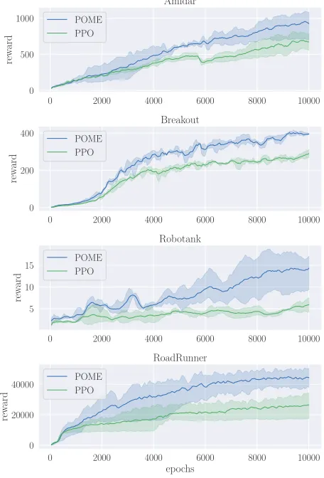
Figure 1: Comparison of POME against PPO on Atari games, training for 10M timesteps, over 3 random seeds.

To estimate the model, due to the fact that learning the state dynamics is more important than learning the rewards, we use a convolutional neural network with one hidden layer to fit the state transition. The inputs of the transition network have two parts, the state (images of four frames) and the ac-tion (a discrete number). Before being fed into the model, the images are scaled to the range [0,1], and the action is one-hot encoded. We concatenate the one-hot encoding of the action to the states’ images to form the inputs of the tran-sition model. We use thesigmoid activation for the outputs of the transition network. After that, we can finally compute the loss function of the transition model between the scaled images of the next state and the outputs.

In the actual implementation, POME use a unified objec-tive function in order to simplify the computation

L=−LPOME(θ) +cvLv(φ) +cTLT(θ_Tˆ), (31)

which is optimized by the Adam gradient descent optimizer (Kingma and Ba 2014) with learning rate2.5×10−4_×f, wheref is a fraction linearly annealed from 1 to 0 over the

Table 1: Comparison between the original PPO and POME with decaying exploration coefficient. The scores of PPO are from the original paper (Schulman et al. 2017)

GAMES PPO POME

Alien 1850.3 1897.0

Amidar 674.6 943.9

Assault 4971.9 5638.6

Asterix 4532.5 4989.2

Asteroids 2097.5 1737.6

Atlantis 2311815.0 1941792.3

BankHeist 1280.6 1241.7

BattleZone 17366.7 15156.7

BeamRider 1590.0 1815.7

Bowling 40.1 58.3

Boxing 94.6 92.9

Breakout 274.8 411.8

Centipede 4386.4 2921.6

ChopperCommand 3516.3 4689.0

CrazyClimber 110202.0 115282.0

DemonAttack 11378.4 14847.1

DoubleDunk -14.9 -6.8

Enduro 758.3 835.3

FishingDerby 17.8 21.1

Freeway 32.5 33.0

Frostbite 314.2 272.9

Gopher 2932.9 4801.8

Gravitar 737.2 914.5

IceHockey -4.2 -4.5

Jamesbond 560.7 507.2

Kangaroo 9928.7 2511.0

Krull 7942.3 8001.1

KungFuMaster 23310.3 24570.3

MontezumaRevenge 42.0 0.0

MsPacman 2096.5 1966.5

NameThisGame 6254.9 5902.2

Pitfall -32.9 -0.3

Pong 20.7 20.8

PrivateEye 69.5 100.0

Qbert 14293.3 15712.8

Riverraid 8393.6 8407.9

RoadRunner 25076.0 44520.0

Robotank 5.5 14.6

Seaquest 1204.5 1789.7

SpaceInvaders 942.5 964.2

StarGunner 32689.0 44696.7

Tennis -14.8 -15.5

TimePilot 4232.0 4052.0

Tutankham 254.4 199.8

UpNDown 95445.0 181250.4

Venture 0 2.0

VideoPinball 37389.0 33388.0

WizardOfWor 4185.3 4301.7

Zaxxon 5008.7 6358.0

Comparison with PPO

Table 1 compares POME with decaying coefficientαagainst the original PPO, on the averaged scores of the last 100 episodes of algorithms with each environment. In Table 1, we see that, among the 49 games, POME with decaying coefficientαoutperforms PPO in 32 games at the last 100 episodes.

The learning curves of four representative Atari games is shown in Figure 1. It shows that, in these environments, POME outperforms PPO over the entire training period, which indicates that it achieves fast learning and validate the power of our exploration technique by using the discrepancy of targets as exploration value.

Additional Experimental Results

We now investigate two questions: (1) how would POME perform if we do not tune the coefficient to0? (2) how would the direct model-based extension of PPO perform?

For the first question, we set up the experiment to see if the exploration value used in POME would damage the per-formance in a long run. The coefficientαis now set to0.1for the entire training period. Secondly, we implement a model-based extension of PPO with the same architecture of the transition network as POME and replacing the target value with the model-based target value (21), so the agent can per-form on-policy learning while maintaining the belief model. We test the two extensions on Atari 2600 games. The setup of the environments and the hyper-parameters remain the same with the previous experiments.

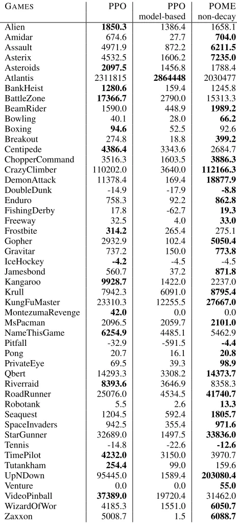
The experimental results in Table 2 show that the model-based version is far from good. Only in one game can it out-performs the baseline. It shows that by using pure model-based PPO, the approximation errors introduced by fitting the model can substantially affect the performance.

However, POME with non-decaying coefficient turns out to be not only good but even better than POME with decay-ing coefficient. It outperforms the original PPO in 33 games out of 49. This result indicates that even though adding the exploration value would increase the bias when estimating the advantage functions, it is empirically not harmful to the policy optimization algorithms in most of the environments.

Conclusion and Discussion

Due to the challenge of the trade-off between exploration and exploitation in environments with continuous state space, in this paper, we propose a novel policy-based algo-rithm named POME, which uses the discrepancy between both target values of model-free and model-based methods to build a relative measure of the exploration value. POME uses several practical techniques to enable the exploration while being stable, i.e., the clipped and centralized explo-ration value. In the actual algorithm, POME builds on the model-free PPO algorithm and adds the exploration bonus to the estimation of the advantage function. Experiments show that POME outperforms the original PPO in 33 Atari games out of 49.

There is yet a limitation that, if the reward signal is ex-tremely sparse, the error of the target values would be close

Table 2: Comparison among PPO, POME with constant ex-ploration coefficient, and the model-based extension of PPO.

GAMES PPO PPO POME

model-based non-decay

Alien 1850.3 1386.4 1658.1

Amidar 674.6 27.7 704.0

Assault 4971.9 872.2 6211.5

Asterix 4532.5 1606.2 7235.0

Asteroids 2097.5 1456.8 1788.4

Atlantis 2311815 2864448 2030477

BankHeist 1280.6 159.4 1245.8

BattleZone 17366.7 2790.0 15313.3

BeamRider 1590.0 448.9 1989.2

Bowling 40.1 28.0 66.2

Boxing 94.6 52.5 92.6

Breakout 274.8 18.8 399.2

Centipede 4386.4 3343.6 2684.7

ChopperCommand 3516.3 1603.5 3886.3

CrazyClimber 110202.0 3640.0 112166.3

DemonAttack 11378.4 169.4 18877.9

DoubleDunk -14.9 -17.9 -8.8

Enduro 758.3 92.2 862.8

FishingDerby 17.8 -62.7 19.3

Freeway 32.5 4.0 33.0

Frostbite 314.2 265.4 275.1

Gopher 2932.9 102.4 5050.4

Gravitar 737.2 150.0 773.8

IceHockey -4.2 -4.5 -4.5

Jamesbond 560.7 37.2 871.8

Kangaroo 9928.7 1422.0 2237.0

Krull 7942.3 6091.0 8795.4

KungFuMaster 23310.3 12255.5 27667.0

MontezumaRevenge 42.0 0.0 0.0

MsPacman 2096.5 2059.7 2101.0

NameThisGame 6254.9 4485.1 5462.9

Pitfall -32.9 -591.5 -4.4

Pong 20.7 16.1 20.8

PrivateEye 69.5 39.3 98.9

Qbert 14293.3 3308.2 14373.7

Riverraid 8393.6 3646.9 8358.3

RoadRunner 25076.0 4534.5 41740.7

Robotank 5.5 2.6 13.3

Seaquest 1204.5 592.4 1805.7

SpaceInvaders 942.5 355.4 971.6

StarGunner 32689.0 1497.5 33836.0

Tennis -14.8 -22.6 -12.6

TimePilot 4232.0 3150.0 3970.7

Tutankham 254.4 99.0 159.6

UpNDown 95445.0 1589.4 203080.4

Venture 0.0 0.0 55.0

VideoPinball 37389.0 19720.4 31462.0

WizardOfWor 4185.3 1551.0 6050.7

Zaxxon 5008.7 1.5 6088.7

References

Auer, P.; Cesa-Bianchi, N.; and Fischer, P. 2002. Finite-time anal-ysis of the multiarmed bandit problem. Machine learning 47(2-3):235–256.

Bellemare, M. G.; Naddaf, Y.; Veness, J.; and Bowling, M. 2013. The arcade learning environment: An evaluation platform for gen-eral agents.Journal of Artificial Intelligence Research47:253–279. Cai, Q.; Filos-Ratsikas, A.; Tang, P.; and Zhang, Y. 2018a. Rein-forcement mechanism design for e-commerce. InProceedings of the 2018 World Wide Web Conference on World Wide Web, 1339– 1348.

Cai, Q.; Filos-Ratsikas, A.; Tang, P.; and Zhang, Y. 2018b. Reinforcement mechanism design for fraudulent behaviour in e-commerce. InProceedings of the 32nd AAAI Conference on Artifi-cial Intelligence.

Cai, Q.; Pan, L.; and Tang, P. 2018. Generalized deterministic policy gradient algorithms.arXiv preprint arXiv:1807.03708. Chen, R. Y.; Sidor, S.; Abbeel, P.; and Schulman, J. 2017. UCB exploration via Q-ensembles.arXiv preprint arXiv:1706.01502. Dhariwal, P.; Hesse, C.; Klimov, O.; Nichol, A.; Plappert, M.; Rad-ford, A.; Schulman, J.; Sidor, S.; Wu, Y.; and Zhokhov, P. 2017. Openai baselines. https://github.com/openai/baselines.

Gu, S.; Lillicrap, T.; Sutskever, I.; and Levine, S. 2016. Continuous deep Q-learning with model-based acceleration. InInternational Conference on Machine Learning, 2829–2838.

Houthooft, R.; Chen, X.; Duan, Y.; Schulman, J.; De Turck, F.; and Abbeel, P. 2016. Vime: Variational information maximizing ex-ploration. InAdvances in Neural Information Processing Systems, 1109–1117.

Kakade, S., and Langford, J. 2002. Approximately optimal ap-proximate reinforcement learning. InICML, volume 2, 267–274. Kingma, D. P., and Ba, J. 2014. Adam: A method for stochastic optimization. InInternational Conference on Learning Represen-tations.

Kurutach, T.; Clavera, I.; Duan, Y.; Tamar, A.; and Abbeel, P. 2018. Model-ensemble trust-region policy optimization. InInternational Conference on Learning Representations.

Levine, S., and Koltun, V. 2013. Guided policy search. In Interna-tional Conference on Machine Learning, 1–9.

Li, W., and Todorov, E. 2004. Iterative linear quadratic regulator design for nonlinear biological movement systems. InICINCO (1), 222–229.

Li, L.; Chu, W.; Langford, J.; and Schapire, R. E. 2010. A contextual-bandit approach to personalized news article recom-mendation. InProceedings of the 19th international conference on World wide web, 661–670.

Lillicrap, T. P.; Hunt, J. J.; Pritzel, A.; Heess, N.; Erez, T.; Tassa, Y.; Silver, D.; and Wierstra, D. 2015. Continuous control with deep reinforcement learning.arXiv preprint arXiv:1509.02971. May, B. C.; Korda, N.; Lee, A.; and Leslie, D. S. 2012. Opti-mistic bayesian sampling in contextual-bandit problems. Journal of Machine Learning Research13(Jun):2069–2106.

Mnih, V.; Kavukcuoglu, K.; Silver, D.; Rusu, A. A.; Veness, J.; Bellemare, M. G.; Graves, A.; Riedmiller, M.; Fidjeland, A. K.; Ostrovski, G.; et al. 2015. Human-level control through deep rein-forcement learning.Nature518(7540):529.

Mnih, V.; Badia, A. P.; Mirza, M.; Graves, A.; Lillicrap, T.; Harley, T.; Silver, D.; and Kavukcuoglu, K. 2016. Asynchronous methods for deep reinforcement learning. InInternational conference on machine learning, 1928–1937.

Montgomery, W. H., and Levine, S. 2016. Guided policy search via approximate mirror descent. InAdvances in Neural Information Processing Systems, 4008–4016.

Pathak, D.; Agrawal, P.; Efros, A. A.; and Darrell, T. 2017. Curiosity-driven exploration by self-supervised prediction. In

International Conference on Machine Learning (ICML), volume 2017.

Peters, J., and Schaal, S. 2006. Policy gradient methods for robotics. InIntelligent Robots and Systems, 2006 IEEE/RSJ In-ternational Conference on, 2219–2225. IEEE.

Schulman, J.; Levine, S.; Abbeel, P.; Jordan, M.; and Moritz, P. 2015. Trust region policy optimization. InInternational Confer-ence on Machine Learning, 1889–1897.

Schulman, J.; Wolski, F.; Dhariwal, P.; Radford, A.; and Klimov, O. 2017. Proximal policy optimization algorithms. InInternational Conference on Learning Representations.

Sutton, R. S., and Barto, A. G. 1998. Reinforcement learning: An introduction, volume 1. MIT press Cambridge.

Sutton, R. S.; McAllester, D. A.; Singh, S. P.; and Mansour, Y. 2000. Policy gradient methods for reinforcement learning with function approximation. InAdvances in neural information pro-cessing systems, 1057–1063.

Sutton, R. S. 1990. Integrated architectures for learning, planning, and reacting based on approximating dynamic programming. In

Machine Learning Proceedings 1990. Elsevier. 216–224. Tang, H.; Houthooft, R.; Foote, D.; Stooke, A.; Chen, O. X.; Duan, Y.; Schulman, J.; DeTurck, F.; and Abbeel, P. 2017. # exploration: A study of count-based exploration for deep reinforcement learn-ing. InAdvances in Neural Information Processing Systems, 2753– 2762.

Tang, P. 2017. Reinforcement mechanism design. InProceedings of the Twenty-Sixth International Joint Conference on Artificial In-telligence, IJCAI-17, 5146–5150.

Thompson, W. R. 1933. On the likelihood that one unknown prob-ability exceeds another in view of the evidence of two samples.

Biometrika25(3/4):285–294.

Wahlstr¨om, N.; Sch¨on, T. B.; and Desienroth, M. P. 2015. From pixels to torques: Policy learning with deep dynamical models. In

Deep Learning Workshop at the 32nd International Conference on Machine Learning.

Wang, Z.; Bapst, V.; Heess, N.; Mnih, V.; Munos, R.; Kavukcuoglu, K.; and de Freitas, N. 2016. Sample efficient actor-critic with experience replay.arXiv preprint arXiv:1611.01224.