A Survey of Algorithms and Analysis
for Adaptive Online Learning
H. Brendan McMahan
[email protected] Google, Inc.
651 N 34th St
Seattle, WA 98103 USA
Editor:Shie Mannor
Abstract
We present tools for the analysis of Follow-The-Regularized-Leader (FTRL), Dual Averaging, and Mirror Descent algorithms when the regularizer (equivalently, prox-function or learning rate schedule) is chosen adaptively based on the data. Adap-tivity can be used to prove regret bounds that hold on every round, and also allows for data-dependent regret bounds as in AdaGrad-style algorithms (e.g., Online Gradient Descent with adaptive per-coordinate learning rates). We present results from a large number of prior works in a unified manner, using a modular and tight analysis that isolates the key arguments in easily re-usable lemmas. This approach strengthens previously known FTRL analysis techniques to produce bounds as tight as those achieved by potential functions or primal-dual analysis. Further, we prove a general and exact equivalence between adaptive Mirror Descent algorithms and a corresponding FTRL update, which allows us to analyze Mirror Descent algorithms in the same framework. The key to bridging the gap between Dual Av-eraging and Mirror Descent algorithms lies in an analysis of the FTRL-Proximal algorithm family. Our regret bounds are proved in the most general form, holding for arbitrary norms and non-smooth regularizers with time-varying weight.
Keywords: online learning, online convex optimization, regret analysis, adaptive algorithms, follow-the-regularized-leader, mirror descent, dual averaging
1. Introduction
We consider the problem of online convex optimization over a series of roundst ∈ {1,2, . . .}. On each round the algorithm selects a point (e.g., a predictor or an action) xt ∈ Rn, and then an adversary selects a convex loss function ft, and the algorithm suffers lossft(xt). The goal is to minimize
RegretT(x∗, ft)≡ T
X
t=1
ft(xt)− T
X
t=1
ft(x∗), (1)
c
Algorithm 1 General Template for Adaptive FTRL
Parameters: Scheme for selecting convex rts.t. ∀x, rt(x)≥0 fort= 0,1,2, . . . x1←arg minx∈Rn r0(x)
for t= 1,2, . . .do
Observe convex loss functionft:Rn→R∪ {∞}
Incur lossft(xt)
Choose incremental convex regularizerrt, possibly based onf1, . . . ft Update
xt+1 ←arg min x∈Rn
t
X
s=1
fs(x) + t
X
s=0 rs(x)
end for
the difference between the algorithm’s loss and the loss of a fixed pointx∗, potentially chosen with full knowledge of the sequence of ft up through round T. When the functions ft and round T are clear from the context we write Regret(x∗). The “adversary” choosing the ft need not be malicious, for example the ft might be drawn from a distribution. The name “online convex optimization” was introduced by Zinkevich (2003), though the setting was introduced earlier by Gordon (1999). When a particular set of comparatorsX is fixed in advance, one is often interested in Regret(X)≡supx∗∈XRegret(x∗); sinceX is often a norm ball, frequently we bound
Regret(x∗) by a function of kx∗k.
Online algorithms with good regret bounds (that is, bounds that are sublinear in T) can be used for a wide variety of prediction and learning tasks (Cesa-Bianchi and Lugosi, 2006; Shalev-Shwartz, 2012). The case of online logistic regression, where one predicts the probability of a binary outcome, is typical. Here, on each round a feature vectorat∈Rnarrives, and we make a predictionpt=σ(at·xt)∈(0,1) using the current model coefficients xt ∈ Rn, where σ(z) = 1/(1 +e−z). The adversary
then reveals the true outcome yt ∈ {0,1}, and we measure loss with the negative log-likelihood, `(pt, yt) = −ytlogpt−(1−yt) log(1−pt). We encode this problem as online convex optimization by taking ft(x) =`(σ(at·x), yt); these ft are in fact convex. Linear Support Vector Machines (SVMs), linear regression, and many other learning problems can be encoded in a similar manner; Shalev-Shwartz (2012) and many of the other works cited here contain more details and examples.
we allow the regularizer to change adaptively. Given a sequence of incremental regularization functionsr0, r1, r2, . . ., we consider the algorithm that selects
x1 ∈arg min x∈Rn
r0(x)
xt+1= arg min x∈Rn
f1:t(x) +r0:t(x) fort= 1,2, . . . , (2)
where we use the compressed summation notationf1:t(x) =Pts=1fs(x) (we also use this notation for sums of scalars or vectors). The argmin in Eq. (2) is over allRn,
but it is often necessary to constrain the selected pointsxt to a convex feasible set
X. This can be accomplished in our framework by including the indicator function IX as a term in r0 (IX is a convex function defined by IX(x) = 0 for x ∈ X and ∞ otherwise); details are given in Section 2.4. The algorithms we consider are adaptive in that each rt can be chosen based on f1, f2, . . . , ft. For convenience, we define functionsht by
h0(x) =r0(x)
ht(x) =ft(x) +rt(x) fort= 1,2, . . .
soxt+1 = arg minxh0:t(x). Generally we will assume the ft are convex, and the rt are chosen so that r0:t (or h0:t) is strongly convex for all t, e.g., r0:t(x) = 21ηtkxk22 (Sections 2.3 and 4.2 review important definitions and results from convex analysis). FTRL algorithms generalize the Follow-The-Leader (FTL) approach (Hannan, 1957; Kalai and Vempala, 2005), which selects xt+1 = arg minxf1:t(x). FTL can provide sublinear regret in the case of strongly convex functions (as we will show), but for general convex functions additional regularization is needed.
Adaptive regularization can be used to construct practical algorithms that pro-vide regret bounds that hold on all roundsT, rather than only on a single roundT which is chosen in advance. The framework is also particularly suitable for analyz-ing AdaGrad-style algorithms that adapt their regularization or norms based on the observed data, for example those of McMahan and Streeter (2010) and Duchi et al. (2010a, 2011). This approach leads to regret bounds that depend on the actual ob-served sequence of functionsft(usually via Oft(xt)), rather than purely worst-case bounds. These tighter bounds translate to much better performance in practice, es-pecially for high-dimensional but sparse problem (e.g., bag-of-words feature vectors). Examples of such algorithms are analyzed in Sections 3.4 and 3.5.
We also study Mirror Descent algorithms, for example updates like
xt+1 = arg min x∈X O
ft(xt)·x+λkxk1+ 1 2ηt
kx−xtk22
whereηtis an adaptive non-increasing learning rate. This update generalizes Online Gradient Descent with a non-smooth regularization term; Mirror Descent also en-compasses the use of an arbitrary Bregman divergence in place of thek · k2
above. We will discuss this family of algorithms at length in Section 6. In fact, Mirror Descent algorithms can be expressed as particular members of the FTRL family, though generally not the most natural ones. In particular, since the state maintained by Mirror Descent is essentially only the current feasible pointxt, we will see that Mirror Descent algorithms are forced to linearize penalties likeλkxk1 from previous rounds, while the more natural FTRL algorithms can keep these terms in closed form, leading to practical advantages such as producing sparser models when L1 regularization is used.
While we focus on online algorithms and regret bounds, the development of many of the algorithms considered rests heavily on work in general convex optimization and stochastic optimization. As a few starting points, we refer the reader to Nemirovsky and Yudin (1983) and Nesterov (2004, 2007). Going the other way, the algorithms presented here can be applied to batch optimization problems of the form
arg min x∈Rn
F(x) where F(x)≡
T
X
t=1
ft(x) (3)
by running the online algorithm for one or more passes over the set offtand return-ing a suitable point (usually the last xt or an average of past xt). Using online-to-batch conversion techniques (e.g., Cesa-Bianchi et al. (2004), Shalev-Shwartz (2012, Chapter 5)), one can convert the regret bounds given here to convergence bounds for the batch problem. Many state-of-the-art algorithms for batch optimization over very large datasets can be analyzed in this fashion.
Outline In Section 2, we elaborate on the family of algorithms encompassed by the update of Eq. (2). We then state two regret bounds, Theorems 1 and 2, which are flexible enough to cover many known results for general and strongly convex functions; in Section 3 we use them to derive concrete bounds for many standard online algorithms.
In Section 4 we break the analysis of adaptive FTRL algorithms into three main components, which helps to modularize the arguments. In Section 4.1 we prove the Strong FTRL Lemma which lets us express the regret through round T as a regularization term on the comparator x∗, namely r0:T(x∗), plus a sum of per-round stability terms. This reduces the problem of bounding regret to that of bounding these per-round terms. In Section 4.2 we review some standard results from convex analysis, and prove lemmas that make bounding the per-round terms relatively straightforward. The general regret bounds are then proved in Section 4.3 as corollaries of these results.
Algorithm 2General Template for Adaptive Linearized FTRL
Parameters: Scheme for selecting convexrt s.t. ∀x, rt(x)≥0 fort= 0,1,2, . . . z←0∈Rn //Maintains g
1:t x1 ←arg minx∈Rn z·x+r0(x) for t= 1,2, . . . do
Select xt, observe loss function ft, incur lossft(xt) Compute a subgradient gt∈∂ft(xt)
Choose incremental convex regularizer rt, possibly based ong1, . . . , gt z←z+gt
xt+1 ←arg minx∈Rn z·x+r0:t(x) //Often solved in closed form end for
equivalence of an arbitrary adaptive Mirror Descent algorithm and a certain FTRL algorithm, and uses this to prove regret bounds for Mirror Descent.
New Contributions The principal goal of this work is to provide a useful sur-vey of central results in the analysis of adaptive algorithms for online convex opti-mization; whenever possible we provide precise references to earlier results that we re-prove or strengthen. Achieving this goal in a concise fashion requires some new results, which we summarize here.
The FTRL style of analysis is both modular and intuitive, but in previous work resulted in regret bounds that are not the tightest possible; we remedy this by introducing the Strong FTRL Lemma in Section 4.1. This also relates the FTRL analysis technique to the primal-dual style of analysis.
By analyzing both FTRL-Proximal algorithms (introduced in the next section) and Dual Averaging algorithms in a unified manner, it is much easier to contrast the strengths and weaknesses of each approach. This highlights a technical but important “off-by-one” difference between the two families in the adaptive setting, as well as an important difference when the algorithm is unconstrained (anyxt∈Rn
is feasible).
Perhaps the most significant new contribution is given in Section 6, where we show that Mirror Descent algorithms (including adaptive algorithms for composite objectives) are in fact particular instances of the FTRL-Proximal algorithm schema, and can be analyzed using the general tools developed for the analysis of FTRL.
2. The FTRL Algorithm Family and General Regret Bounds
Second, we consider whether the incremental regularizers rt are all minimized at a fixed stationary point x1, or are chosen so they are minimized at the current xt. After discussing these options, we state general regret bounds.
2.1 Linearization and the Optimization of Lower Bounds
In practice, it may be infeasible to solve the optimization problem of Eq. (2), or even represent it as t becomes sufficiently large. A key point is that we can derive a wide variety of first-order algorithms by linearizing the ft, and running the algorithm on these linear functions. Algorithm 2 gives the general scheme. For convex ft, let xt be defined as above, and let gt ∈ ∂ft(xt) be a subgradient (e.g., gt= Oft(xt) for differentiable ft). Convexity implies for any comparator x∗, ft(xt)−ft(x∗) ≤gt·(xt−x∗). A key observation of Zinkevich (2003) is that if we let ¯ft(x) = gt·x, then for any algorithm the regret against the functions ¯ft upper bounds the regret against the originalft:
Regret(x∗, ft)≤Regret(x∗,f¯t).
Note we can construct the functions ¯ft on the fly (after observing xt and ft) and then present them to the algorithm.
Thus, rather than solving xt+1 = arg minxf1:t(x) + r0:t(x) on each round t, we now solve xt+1 = arg minxg1:t·x+r0:t(x). Note that g1:t ∈ Rn, and we will
generally choose the rt so that r0:t(x) can also be represented in constant space. Thus, we have at least ensured our storage requirements stay constant even as t → ∞. Further, we will usually be able to choose rt so the optimization with g1:t can be solved in closed form. For example, if we taker0:t(x) = 21ηkxk22 then we can solvext+1 = arg minxg1:t·x+r0:t(x) in closed form, yieldingxt+1 =−ηg1:t(that is, this FTRL algorithm is exactly constant learning rate Online Gradient Descent). However, we will usually state our results in terms of general ft, since one can always simply take ft = ¯ft when appropriate. In fact, an important aspect of our analysis is that it does not depend on linearization; our regret bounds hold for the the general update of Eq. (2) as well as applying to linearized variants.
More generally, we can run the algorithm on any ¯ftthat satisfy ¯ft(xt)−f¯t(x∗)≥ ft(xt)−ft(x∗) for all x∗ and have the regret bound achieved for the ¯f also apply to the original f. This is generally accomplished by constructing a lower bound ¯ft that is tight at xt, that is ¯ft(x) ≤ ft(x) for all x and further ¯ft(xt) = ft(xt). A tight linear lower bound is always possible for convex functions, but for example if the ft are all strongly convex, better algorithms are possible by taking ¯ft to be an appropriate quadratic lower bound.
convex functions”) is distinct from the modeling decision to replace a non-convex loss function (e.g., the zero-one loss for classification) with a convex upper bound (e.g., the hinge loss). This “convexification by surrogate loss” approach is described in detail by (Shalev-Shwartz, 2012, Sec 2.1).
2.2 Regularization in FTRL Algorithms
The term “regularization” can have multiple meanings, and so in this section we clarify the different roles regularization plays in the present work.
We refer to the functionsr0:tas regularization functions, withrtthe incremental increase in regularization on round t (we assume rt(x) ≥ 0). This is the regular-ization in the name Follow-The-Regularized-Leader, and these rt terms should be viewed as part of the algorithm itself—analogous (and in some cases exactly equiv-alent) to the learning rate schedule in an Online Gradient Descent algorithm, for example. The adaptive choice of these regularizers is the principle topic of the current work. We study two main classes of regularizers:
• InFTRL-Centered algorithms, eachrt(and hence r0:t) is minimized at a fixed point, x1 = arg minxr0(x). An example is Dual Averaging (which also lin-earizes the losses), where r0:t is called theprox-function (Nesterov, 2009).
• In FTRL-Proximal algorithms, each incremental regularization functionrt is minimized by xt, and we call such rt incremental proximal regularizers.
When we make neither a proximal nor centered assumption on the rt, we refer to general FTRL algorithms. Theorem 1 (below) allows us to analyze regularization choices that do not fall into either of these two categories, but the Centered and Proximal cases cover the algorithms of practical interest.
There are a number of reasons we might wish to add additional regularization terms to the objective function in the FTRL update. In many cases this is handled immediately by our general theory by grouping the additional regularization terms with either theftor thert. However, in some cases it will be advantageous to handle this additional regularization more explicitly. We study this situation in detail in Section 5.
2.3 General Regret Bounds
In this section we introduce two general regret bounds that can be used to analyze many different adaptive online algorithms. First, we introduce some additional notation and definitions.
Notation and Definitions An extended-value convex functionψ:Rn→R∪{∞}
satisfies
forθ∈(0,1), and the domain ofψ is the convex set domψ≡ {x:ψ(x)<∞}(e.g., Boyd and Vandenberghe (2004, Sec. 3.1.2)); ψis proper if∃x∈Rn s.t.ψ(x)<+∞ and ∀x ∈Rn, ψ(x) >−∞. We refer to extended-value proper convex functions as
simply “convex functions.”
We write∂ψ(x) for the subdifferential ofψatx; a subgradientg∈∂ψ(x) satisfies
∀y∈Rn, ψ(y)≥ψ(x) +g·(y−x).
The subdifferential ∂ψ(x) for a convex ψ is always non-empty for x ∈int (domψ), and typically non-empty for any x ∈ domψ for the functions ψ considered in this work; ∂ψ(x) is empty for x6∈domψ(Rockafellar, 1970, Thm. 23.2).
Working with extended convex functions lets us encode constraints seamlessly by using IX, the indicator function on a convex set X ⊆Rn given by
IX(x) = (
0 x∈ X
∞ otherwise , (4)
since IX is itself an extended convex function. Generally we assume X is a closed convex set. This approach makes it convenient to write arg minx as shorthand for arg minx∈Rn.
A function ψ :Rn→ R∪ {∞}is σ-strongly convex w.r.t. a normk · k if for all
x, y∈Rn,
∀g∈∂ψ(x), ψ(y)≥ψ(x) +g·(y−x) +σ2ky−xk2. (5) If some ψ only satisfies Eq. (5) for x, y ∈ X for a convex set X, then the function ψ0 = ψ+IX satisfies Eq. (5) for all x, y ∈ Rn, and so is strongly convex by our definition. Thus, we can work with ψ0 without any need to explicitly refer to X.
The convex conjugate (or Fenchel conjugate) of an arbitrary functionψ:Rn→ R∪ {∞}is
ψ?(g)≡sup x
g·x−ψ(x). (6)
For a norm k · k, the dual norm is given by
kxk?≡ sup y:kyk≤1
x·y.
It follows from this definition that for anyx, y∈Rn,x·y≤ kxkkyk
?, a generalization of H¨older’s inequality. We make heavy use of normsk · k(t)that change as a function of the roundt; the dual norm of k · k(t) isk · k(t),?.
Our basic assumptions correspond to the framework of Algorithm 1, which we summarize together with a few technical conditions as follows:
loss functions ft : Rn → R∪ {∞}. Further, letting h0:t = r0:t+f1:t we assume domh0:tis non-empty. Recalling xt= arg minxh0:t−1(x), we further assume∂ft(xt)
is non-empty.
The minor technical assumptions made here do not rule out any practical applica-tions. We can now introduce the theorems which will be our main focus. The first will typically be applied to FTRL-Centered algorithms such as Dual Averaging:
Theorem 1 General FTRL Bound Consider Setting 1, and suppose the rt are
chosen such that h0:t+ft+1 = r0:t+f1:t+1 is 1-strongly-convex w.r.t. some norm k · k(t). Then, for any x∗ ∈Rn and for any T >0,
RegretT(x∗)≤r0:T−1(x∗) + 1 2
T
X
t=1
kgtk2(t−1),?.
Our second theorem handles proximal regularizers:
Theorem 2 FTRL-Proximal BoundConsider Setting 1, and further suppose the rtare chosen such thath0:t=r0:t+f1:tis 1-strongly-convex w.r.t. some normk · k(t), and further thert are proximal, that is xt is a minimizer of rt. Then, choosing any gt∈∂ft(xt) on each round, for anyx∗∈Rn and for any T >0,
RegretT(x∗)≤r0:T(x∗) + 1 2
T
X
t=1
kgtk2(t),?.
We state these bounds in terms of strong convexity conditions on h0:t in order to also cover the case where the ft are themselves strongly convex. In fact, if eachft is strongly convex, then we can choose rt(x) = 0 for all t, and Theorems 1 and 2 produceidentical bounds (and algorithms).1 When it is not known a priori whether the loss functions ft are strongly convex, the rt can be chosen adaptively to add only as much strong convexity as needed, following Bartlett et al. (2007). On the other hand, when theft are not strongly convex (e.g., linear), a sufficient condition for both theorems is choosing thert such thatr0:tis 1-strongly-convex w.r.t. k · k(t). It is worth emphasizing the “off-by-one” difference between Theorems 1 and 2 in this case: we can choose rt based on gt, and when using proximal regularizers, this lets us influence the norm we use to measure gt in the final bound (namely the kgtk2(t),? term); this is not possible using Theorem 1, since we have kgtk2(t−1),?. This makes constructing AdaGrad-style adaptive learning rate algorithms for FTRL-Proximal easier (McMahan and Streeter, 2010), whereas with FTRL-Centered algo-rithms one must start with slightly more regularization. We will see this in more detail in Section 3.
1. To see this, note in Theorem 1 the norm inkgtk(t−1),?is determined by the strong convexity of
Theorem 1 leads immediately to a bound for Dual Averaging algorithms (Nes-terov, 2009), including the Regularized Dual Averaging (RDA) algorithm of Xiao (2009), and its AdaGrad variant (Duchi et al., 2011) (in fact, this statement is equiv-alent to Duchi et al. (2011, Prop. 2) when we assume theftare not strongly convex). As in these cases, Theorem 1 is usually applied to FTRL-Centered algorithms where x1 (often the origin) is a global minimizer of r0:t for each t. The theorem does not require this; however, such a condition is usually necessary to boundr0:T−1(x∗) and hence Regret(x∗) in terms ofkx∗k.
Less general versions of these theorems often assume that eachr0:tisαt -strongly-convex with respect to a fixed normk · k. Our results include this as a special case, see Section 3 and Lemma 3 in particular.
Non-Adaptive Algorithms These theorems can also be used to analyze non-adaptive algorithms. If we chooser0(x) to be a fixed non-adaptive regularizer (per-haps chosen with knowledge of T) that is 1-strongly convex w.r.t. k · k, and all rt(x) = 0 for t ≥ 1, then we have kxk(t),? = kxk? for all t, and so both theorems provide the identical statement
Regret(x∗)≤r0(x∗) + 1 2
T
X
t=1
kgtk2?. (7)
This matches Shalev-Shwartz (2012, Theorem 2.11), though we improve by a con-stant factor due to the use of the Strong FTRL Lemma.
2.4 Incorporating a Feasible Set
We have introduced the FTRL update as an unconstrained optimization over x ∈
Rn. For many learning problems, where xt is a vector of model parameters, this may be fine, but in other applications we need to enforce constraints. These could correspond to budget constraints, structural constraints like kxtk2 ≤R orkxtk1 ≤ R1, a constraint thatxtis a flow on a graph, or thatxtis a probability distribution. In all of these cases, this amounts to the constraint that xt ∈ X where X is a suitable convex feasible set. Further, for FTRL-Proximal algorithms a constraint likekxtk2 ≤R is generally needed in order to boundr0:T(x∗); see Section 3.3.
Such constraints can be addressed immediately in our setting by adding the additional regularizerIX tor0, based on the equivalence
arg min x∈Rn
f1:t(x) +r0:t(x) +IX(x) = arg min x∈X
f1:t(x) +r0:t(x).
Note that while the theorems still apply, the regret bounds change in an im-portant way, since IX(x∗) now appears in the regret bound: that is, if Theorem 1 on functionsr0, r1, . . . , gives a bound Regret(x∗)≤r0:T−1(x∗) +12PTt=1kgtk2(t−1),?, then the version constrained to select fromX by addingIX tor0 has regret bound
RegretT(x∗)≤IX(x∗) +r0:T−1(x∗) + 1 2
T
X
t=1
kgtk2(t−1),?.
This bound is vacuous for x∗ 6∈ X, but identical to the unconstrained bound for x∗ ∈ X. This makes sense: one can show that any online algorithm constrained to select xt ∈ X cannot in general hope to have sublinear regret against some x∗ 6∈ X. Thus, if we believe some x∗ 6∈ X could perform very well, incorporating the constraintxt∈ X is a significant sacrifice that should only be made if external considerations really require it.
3. Application to Specific Algorithms and Settings
Before proving these theorems, we apply them to a variety of specific algorithms. We will use the following lemma, which collects some facts for the sequence of incremental regularizersrt. These claims are immediate consequences of the relevant definitions.
Lemma 3 Consider a sequence ofrtas in Setting 1. Then, sincert(x)≥0, we have r0:t(x) ≥r0:t−1(x), and so r0:?t(x) ≤r0:?t−1(x), where r0:?t is the convex-conjugate of r0:t. If each rt is σt-strongly convex w.r.t. a norm k · k for σt ≥ 0, then, r0:t is σ0:t-strongly convex w.r.t. k · k, or equivalently, is 1-strongly-convex w.r.t. kxk(t) = √
σ0:tkxk, which has dual norm kxk(t),?= √σ10:tkxk.
For reasons that will become clear, it is natural to define a learning rate scheduleηt to be the inverse of the cumulative strong convexity,
ηt= 1 σ0:t
.
In fact, in many cases it will be more natural to define the learning rate schedule, and infer the sequence ofσt,
σt= 1 ηt
− 1 ηt−1
,
withσ0 = η10.
3.1 Constant Learning Rate Online Gradient Descent
As a warm-up, we first consider a non-adaptive algorithm, unconstrained constant learning rate Online Gradient Descent, which selects x1 = 0 and thereafter
xt+1=xt−ηgt, (8) where the parameterη >0 is the learning rate. Iterating this update, we seext+1 = −ηg1:t. There is a close connection between Online Gradient Descent and FTRL, which we will use to analyze this algorithm. If we take FTRL with r0(x) = 21ηkxk2 2 and rt(x) = 0 for t≥1, we have the update
xt+1 = arg min x
g1:t·x+ 1 2ηkxk
2
2, (9)
which we can solve in closed form to see xt+1 = −ηg1:t as well. Applying either Theorem 1 or 2 (recall they are equivalent when the regularizer is fixed) gives the bound of Eq. (7), in this case
RegretT(x∗)≤ 1 2ηkx
∗k2 2+
1 2
T
X
t=1
ηkgtk22, (10)
using Lemma 3 for kxk(t),? = √ηkxk2. Suppose we are concerned with x∗ where kx∗k2 ≤ R, the gt satisfy kgtk2 ≤ G, and we want to minimize regret after T0 rounds. Then, choosing η= R
G√T0 minimizes Eq. (10) when T =T
0, and we have
RegretT(x∗)≤ RG 2
√
T0+RG 2
T √
T0,
or Regret(x∗) ≤RG√T when T = T0. However, this bound is only O(√T) when T =O(T0). For T T0, or T T0 the bound is no longer interesting, and in fact the algorithm will likely perform poorly. This deficiency can be addressed via the “doubling trick”, where we double T0 and restart the algorithm each timeT grows larger than T0 (c.f., Shalev-Shwartz (2012, 2.3.1)). However, adaptively choosing the learning rate without restarting will allow us to achieve better bounds than the doubling trick (by a constant factor) with a more practically useful algorithm. We do this in Sections 3.2 and 3.3 below.
Constant Learning Rate Online Gradient Descent with a Feasible Set Above we assumed kx∗k2 ≤ R, but there is no a priori bound on the magnitude of the xt selected by the algorithm. Following the approach of Section 2.4, we can incorporate a feasible set by taking r0(x) = 21ηkxk2
2+IX(x),so the update becomes xt+1 = arg min
x∈Rn
g1:t·x+ 1 2ηkxk
2
2+IX(x) = arg min x∈X
g1:t·x+ 1 2ηkxk
Following Shalev-Shwartz (2012, Sec. 2.6), this update is equivalent to the two-step update where we first solve the unconstrained problem and then project onto the feasible set, namely
ut+1 = arg min x∈Rn
g1:t·x+ 1 2ηkxk
2 2
xt+1 = ΠX(ut+1) where ΠX(u)≡arg min x∈X
kx−uk2.
Many FTRL algorithms on feasible sets can in this way be interpreted as lazy-projection algorithms, where we find (or maintain) the solution to the unconstrained problem, and then project onto the feasible set when needed.
Theorem 1 can be used to analyze the constrained algorithm of Eq. (11) in exactly the same way we analyzed Eq. (9): adding IX does not change the strong convexity of thekxk2
2 terms in the regularizer, and so the only difference is in the r0:T(x∗) term. Instead of Eq. (10), we have
∀x∗∈ X, RegretT(x∗)≤ 1 2ηkx
∗k2 2+
1 2
T
X
t=1
ηkgtk22,
where we have chosen to use the explicit∀x∗ ∈ X rather than the equivalent choice of includingIX(x∗) on the right-hand side.
Interestingly, the update of Eq. (11) is no longer equivalent to the standard pro-jected Online Gradient Descent updatext+1 = ΠX(xt−ηgt); this issue is discussed in the context of more general Mirror Descent updates in Appendix C.2. We will be able to analyze this algorithm using techniques from Section 6.
3.2 Dual Averaging
Dual Averaging is an adaptive FTRL-Centered algorithm with linearized loss func-tions; the adaptivity allows us to prove regret bounds that are O(√T) for all T. We choose rt(x) = σ2tkxk22 for constants σt ≥ 0, so r0:t is 1-strongly-convex w.r.t. the normkxk(t) =√σ0:tkxk2, which has dual normkxk(t),?= √σ10:tkxk2 =
√
ηtkxk2, using Lemma 3. Plugging into Theorem 1 then gives
∀T, RegretT(x∗)≤ 1 2ηT−1
kx∗k22+1 2
T
X
t=1
ηt−1kgtk22.
Suppose we knowkgtk2 ≤G, and we consider x∗ wherekx∗k2 ≤R. Then, with the choiceηt= √2GR√t+1, using the inequality PTt=1 √1t ≤2
√
T, we arrive at
∀T, RegretT(x∗)≤ √
2 2
R+kx ∗k2
2 R
G
√
When in fact kx∗k ≤R, we have Regret≤√2RG√T, but the bound of Eq. (12) is valid (and meaningful) for arbitrary x∗ ∈Rn. Observe that on a particular round T, this bound is a factor√2 worse than the bound ofRG√T shown in Section 3.1 when the learning rate is tuned for exactly roundT; this is the (small) price we pay for a bound that holds uniformly for all T.
As in the previous example, Dual Averaging can also be restricted to select from a feasible set X by including IX in r0. Additional non-smooth regularization can also be applied by adding the appropriate terms to r0 (or any of the rt); for example, we can add an L1 and L2 penalty by adding the terms λ1kxk1+λ2kxk22. When in addition theftare linearized, this produces the Regularized Dual Averaging algorithm of Xiao (2009). Note that our result of√2RG√Timproves on the bound of 2RG√T achieved by Xiao (2009, Cor. 2(a)). We consider the case of such additional regularization terms in more detail in Section 5.
3.3 FTRL-Proximal
Suppose X ⊆ {x | kxk2 ≤R}, and we choose r0(x) =IX(x) and for t >1, rt(x) = σt
2kx−xtk 2
2. It is worth emphasizing that unlike in the previous examples, for FTRL-Proximal the inclusion of the feasible set X is essential to proving regret bounds. With this constraint we haver0:t(x∗)≤ σ1:2t(2R)2for anyx∗ ∈ X, since eachxt∈ X. Without forcingxt∈ X, however, the termskx∗−xtk22 inr0:t(x∗) cannot be usefully bounded.
With these choices, r0:tis 1-strongly-convex w.r.t. the norm kxk(t) = √
σ1:tkxk2, which has dual normkxk(t),? = √1
σ1:tkxk2. Thus, applying Theorem 2, we have
∀x∗ ∈ X, Regret(x∗)≤ 1 2ηT
(2R)2+1 2
T
X
t=1
ηtkgtk2, (13)
where again ηt= σ11:t. Choosingηt= √
2R
G√t and assuming kx
∗k ≤R andkg
tk2≤G, Regret(x∗)≤2√2RG
√
T . (14)
Note that we are a factor of 2 worse than the corresponding bound for Dual Averag-ing. However, this is essentially an artifact of loosely boundingkx∗−xtk22 by (2R)2, whereas for Dual Averaging we can boundkx∗−0k2
2 withR2. In practice one would hope xt is closer to x∗ than 0, and so it is reasonable to believe that the FTRL-Proximal bound will actually be tighter post-hoc in many cases. Empirical evidence also suggests FTRL-Proximal can work better in practice (McMahan, 2011).
3.4 FTRL-Proximal with Diagonal Matrix Learning Rates
first consider a one-dimensional problem. Let r0 =IX withX = [−R, R], and fix a learning rate schedule for FTRL-Proximal where
ηt=
√ 2R q
Pt
s=1g2s for use in Eq. (13). This gives
Regret(x∗)≤2√2R v u u t T X t=1 g2
t, (15)
where we have used the following lemma, which generalizesPT
t=11/ √
t≤2√T:
Lemma 4 For any non-negative real numbers a1, a2, . . . , an, n X i=1 ai q Pi
j=1aj ≤2 v u u t n X i=1 ai .
For a proof see Auer et al. (2002) or Streeter and McMahan (2010, Lemma 1). The bound of Eq. (15) gives us a fully adaptive version of Eq. (14): not only do we not need to know T in advance, we also do not need to know a bound on the norms of the gradients G. Rather, the bound is fully adaptive and we see, for example, that the bound only depends on rounds t where the gradient is nonzero (as one would hope). We do, however, require that R is chosen in advance; for algorithms that avoid this, see Streeter and McMahan (2012); Orabona (2013); McMahan and Abernethy (2013), and McMahan and Orabona (2014).
To arrive at an AdaGrad-style algorithm for n-dimensions we need only apply the above technique on a per-coordinate basis, namely using learning rate
ηt,i =
√ 2R∞ q
Pt
s=1gs,i2
for coordinatei, where we assumeX ⊆[−R∞, R∞]n. Streeter and McMahan (2010) take the per-coordinate approach directly; the more general approach here allows us to handle arbitrary feasible sets andL1 or other non-smooth regularization.
We take r0 = IX, and for t ≥ 1 define rt(x) = 12kQ 1 2
t(x−xt)k22 where Qt = diag σt,i), the diagonal matrix with entriesσt,i =ηt,i−1−η
−1
t−1,i. This Qt is positive semi-definite, and for any such Qt, we have thatr0:t is 1-strongly-convex w.r.t. the norm kxk(t) = k(Q1:t)
1
2xk2, which has dual norm kgk(t),? = k(Q1:t)− 1
2gk2. Then, plugging into Theorem 2 gives
Regret(x∗)≤r0:T(x∗) + 1 2
T
X
t=1
which improves on McMahan and Streeter (2010, Theorem 2) by a constant factor. Essentially, this bound amounts to summing Eq. (15) across all n dimensions; McMahan and Streeter (2010, Cor. 9) show this bound is at least as good (and often better) than that of Eq. (14). Full matrix learning rates can be derived using a matrix generalization of Lemma 4, e.g., Duchi et al. (2011, Lemma 10); however, since this requires O(n2) space and potentially O(n2) time per round, in practice these algorithms are often less useful than the diagonal varieties.
It is perhaps not immediately clear that the diagonal FTRL-Proximal algorithm is easy and efficient to implement. However, taking the linear approximation to ft, one can see h1:t(x) = g1:t·x+r1:t(x) is itself just a quadratic which can be represented using two length n vectors, one to maintain the linear terms (g1:t plus adjustment terms) and one to maintain Pt
s=1gs,i2 , from which the diagonal entries of Q1:tcan be constructed. That is, the update simplifies to
xt+1 = arg min x∈X
(g1:t−a1:t)·x+ n
X
i=1 1 2ηt,i
x2i where at=σtxt.
This update can be solved in closed-form on a per-coordinate basis when X = [−R∞, R∞]n. For a general feasible set, it is equivalent to a lazy-projection algorithm that first solves for the unconstrained solution and then projects it onto X using norm k(Q1:t)
1
2 · k (see McMahan and Streeter (2010, Eq. 7)). Pseudo-code which also incorporatesL1 and L2 regularization is given in McMahan et al. (2013).
3.5 AdaGrad Dual Averaging
Similar ideas can be applied to Dual Averaging (where we center each rt at x1), but one must use some care due to the “off-by-one” difference in the bounds. For example, for the diagonal algorithm, it is necessary to choose per-coordinate learning rates
ηt≈
R q
G2+Pt
s=1g2s ,
where|gt| ≤G. Thus, we arrive at an algorithm that is almost (but not quite) fully adaptive in the gradients, since a modest dependence on the initial guess Gof the maximum per-coordinate gradient remains in the bound. This offset appears, for example, as theδI terms added to the learning rate matrixHtin Figure 1 of Duchi et al. (2011). We will see this issue again in Section 3.7.
3.6 Strongly Convex Functions
Non-Adaptive FTRL Algorithms(fixed regularizerr0, withrt(x) = 0 fort≥1) Constant Learning Rate Unprojected Online Gradient Descent
xt+1=xt−ηgt
= arg min x
g1:t·xt+ 1 2ηkxk
2 2
=−ηg1:t
Follow-The-Leader where theftare 1-strongly-convex w.r.t. k · k
xt+1= arg min x
f1:t(x)
Online Gradient Descent for strongly-convex functions
xt+1= arg min x
g1:t·x+ 1 2
t
X
s=1
kx−xsk2 wheregt∈∂ft(xt)
=xt−ηtgt whereηt= 1
t
Adaptive FTRL-Centered Algorithms(rt chosen adaptively and minimized atx1)
Unconstrained Dual Averaging (adaptive tot)
xt+1= arg min x
g1:t·x+ 1 2ηt
kxk2
2 whereηt=
R √
2G√t+ 1 =−ηtg1:t
FTRL with the entropic regularizer over the probability simplex ∆ (adaptive togt)
xt+1= arg min x∈∆
g1:t·x+ 1 2ηt
n
X
i=1
xilogxi where ηt=
√ logn q G2 ∞+ Pt
s=1kgsk2∞ , or
xt+1,i=
exp(−ηtg1:t,i)
Pn
i=1exp(−ηtg1:t,i)
in closed form
Adaptive FTRL-Proximal Algorithms(rtchosen adaptively and minimized atxt) FTRL-Proximal (adaptive tot) withσs=η−s1−η−
1 s−1
xt+1= arg min x∈X
g1:t·x+ t
X
s=1 σs
2 kx−xsk
2
2 whereηt=
√
2R G√t
AdaGrad FTRL-Proximal (adaptive togt) withσs,i =η−s,i1−η
−1 s−1,i.
xt+1= arg min x∈X
g1:t·x+ t X s=1 1 2 diag σ 1 2 s,i
(x−xs)
2
2
whereηt,i=
√
2R
q Pt
s=1g 2 s,i
√
tkxk, and observe h0:t(x) is 1-strongly-convex w.r.t. k · k(t) (by Lemma 3). Then, applying either Theorem 1 or 2 (recalling they coincide when all rt(x) = 0),
Regret(x∗)≤ 1 2
T
X
t=1
kgtk2(t),?= 1 2
T
X
t=1 1
tkgtk 2 ≤ G2
2 (1 + logT),
where we have used the inequality PT
t=11/t ≤ 1 + logT and assumed kgtk ≤ G. This recovers, e.g., Kakade and Shalev-Shwartz (2008, Cor. 1) for the the exact FTL algorithm. This algorithm requires optimizing overf1:t exactly, which may be computationally prohibitive.
For a 1-strongly-convex ft withgt∈∂ft(xt) we have by definition
ft(x)≥ft(xt) +gt·(x−xt) + 1
2kx−xtk 2
| {z }
= ¯ft
.
Thus, we can define a ¯ft equal to the right-hand-side of the above inequality, so ¯
ft(x)≤ft(x) and ¯ft(xt) =ft(xt). The ¯ftare also 1-strongly-convex w.r.t.k·k, and so running FTL on these functions produces an identical regret bound. Theorem 11 will show that the update xt+1 = arg minxf1:¯ t(x) is equivalent to the Online Gradient Descent update
xt+1 =xt− 1
tgt,
showing this update is essentially the Online Gradient Descent algorithm for strongly convex functions given by Hazan et al. (2007).2
3.7 Adaptive Dual Averaging with the Entropic Regularizer
We consider problems where the algorithm selects a probability distribution (e.g., in order to sample an action from a discrete set ofnchoices), that is xt∈∆nwith
∆n=
n x
Xn
i=1xi = 1 and xi ≥0 o
.
We assume gradients are bounded so thatkgtk∞≤G∞, which is natural for exam-ple if each action has a cost in the range [−G∞, G∞], so gt·x gives the expected cost of choosing an action from the distribution x. This is the classic problem of prediction from expert advice (Vovk, 1990; Littlestone and Warmuth, 1994; Freund and Schapire, 1995; Cesa-Bianchi and Lugosi, 2006).
The previously introduced algorithms can be applied by enforcing the constraint x ∈ ∆n by adding I∆n to r0, but to instantiate their bounds we can only bound
kgtk2 by √
nG∞ in this case, leading to bounds like O(G∞√nT). By using a more appropriate regularizer, we can reduce the dependence on the dimension from√n to√logn. In particular, we use the entropic regularizer,
H(x) =I∆(x) + logn+ n
X
i=1
xilogxi,
from which we define the following adaptive regularization schedule:
r0:t(x) = 1 ηt
H(x) where ηt=
√ logn q G2 ∞+ Pt
s=1kgsk2∞
for t ≥ 0. Note that as in AdaGrad Dual Averaging, we make the learning rate scheduleηt a function of the observed gt. The function H (and hence each r0:t) is minimized by the uniform distributionx1= (1/n, . . . ,1/n) whereH(x) = 0, and so these regularizers are centered at x1. Note also that h is maximized at the corners of ∆n (e.g., x= (1,0, . . . ,0)) where it has value logn.
The entropic regularizerHis 1-strongly-convex with respect to theL1 norm over the probability simplexX (e.g., Shalev-Shwartz (2012, Ex 2.5)), and it follows that r0:t is 1-strongly convex with respect to the norm kxk(t) = √1ηtkxk1, and kgk2(t),? = ηtkgk2∞.Then, applying Theorem 1, we have
Regret(x∗)≤r0:T−1(x∗) + 1 2
T
X
t=1
kgtk2(t−1),?
≤ logn ηT−1
+1 2
T
X
t=1
ηt−1kgtk2∞
≤ logn ηT−1
+ √ logn 2 T X t=1
kgtk2∞ q
Pt
s=1kgsk2∞
since∀t, kgtk∞≤G∞
≤2 v u u
t G2∞+
T−1 X
t=1 kgtk2∞
!
logn Lemma 4 and kgTk∞≤G∞
≤2G∞pTlogn.
4. A General Analysis Technique
In this section, we prove Theorems 1 and 2; the analysis techniques developed will also be used in subsequent sections to analyze composite objectives and Mirror Descent algorithms.
4.1 Inductive Lemmas
In this section we prove the following lemma that lets us analyze arbitrary FTRL-style algorithms:
Lemma 5 (Strong FTRL Lemma) Let ft be a sequence of arbitrary (possibly
non-convex) loss functions, and let rt be arbitrary non-negative regularization
func-tions, such that xt+1 = arg minxh0:t(x) is well defined, where h0:t(x) ≡ f1:t(x) + r0:t(x). Then, the algorithm that selects these xt achieves
Regret(x∗)≤r0:T(x∗) + T
X
t=1
h0:t(xt)−h0:t(xt+1)−rt(xt). (16)
This lemma can be viewed as a stronger form of the more well-known standard FTRL Lemma (see Kalai and Vempala (2005); Hazan (2008), Hazan (2010, Lemma 1), McMahan and Streeter (2010, Lemma 3), and Shalev-Shwartz (2012, Lemma 2.3)). The strong version has three main advantages over the standard version: 1) it is essentially tight, which improves the final bounds by a constant factor, 2) it can be used to analyze adaptive FTRL-Centered algorithms in addition to FTRL-Proximal, and 3) it relates directly to the primal-dual style of analysis. For completeness, in Appendix A we present the standard version of the lemma, along with the proof of a bound analogous to Theorem 2 (but weaker by a constant factor).
The Strong FTRL Lemma bounds regret by the sum of two factors:
• Stability The terms in the sum over t measure how much better xt+1 is for the cumulative objective function h0:t than the point actually selected, xt: namelyh0:t(xt)−h0:t(xt+1). These per-round terms can be seen as measuring the stability of the algorithm, an online analog to the role of stability in the stochastic setting (Bousquet and Elisseeff, 2002; Rakhlin et al., 2005; Shalev-Shwartz et al., 2010).
• Regularization The term r0:T(x∗) quantifies how much regularization we have added, measured at the comparator pointx∗. This captures the intuitive fact that if we could center our regularization at x∗ it should not increase regret.
r0:T(x∗). At the heart of the adaptive algorithms we study is the ability to dynam-ically balance these two competing goals.
The following corollary relates the above statement to the primal-dual style of analysis:
Corollary 6 Consider the same conditions as Lemma 5, and further suppose the loss functions are linear,ft(x) =gt·xt. Then,
h0:t(xt)−h0:t(xt+1)−rt(xt) =r?0:t(−g1:t)−r?0:t−1(−g1:t−1) +gt·xt, (17)
which implies
Regret(x∗)≤r0:T(x∗) + T
X
t=1
r?0:t(−g1:t)−r?0:t−1(−g1:t−1) +gt·xt.
We make a few remarks before proving these results at the end of this section. Corollary 6 can easily be proved directly using the Fenchel-Young inequality. Our statement directly matches the first claim of Orabona (2013, Lemma 1), and in the non-adaptive case re-arrangement shows equivalence to Shalev-Shwartz (2007, Lemma 1) and Shalev-Shwartz (2012, Lemma 2.20); see also Kakade et al. (2012, Corollary 4). McMahan and Orabona (2014, Thm. 1) give a closely related duality result for regret and reward, and discuss several interpretations for this result, in-cluding the potential function view, the connection to Bregman divergences, and an interpretation ofr? as a benchmark target for reward.
Note, however, that Lemma 5 is strictly stronger than Corollary 6: it applies to non-convex ft and rt. Further, even for convex ft, it can be more useful: for example, we can directly analyze strongly convex ft with all rt(x) = 0 using the first statement. Lemma 5 is also arguably simpler, in that it does not require the introduction of convexity or the Fenchel conjugate. We now prove the Strong FTRL Lemma:
include a−h0(x∗) term as well): T
X
t=1
ht(xt)−h0:T(x∗)
= T
X
t=1
(h0:t(xt)−h0:t−1(xt))−h0:T(x∗)
≤
T
X
t=1
(h0:t(xt)−h0:t−1(xt))−h0:T(xT+1) Since xT+1 minimizesh0:T
≤
T
X
t=1
(h0:t(xt)−h0:t(xt+1)),
where the last line follows by simply re-indexing the −h0:t terms and dropping the the non-positive term−h0(x1) =−r0(x1)≤0. Expanding the definition ofhon the left-hand-side of the above inequality gives
T
X
t=1
(ft(xt) +rt(xt))−f1:T(x∗)−r0:T(x∗)≤ T
X
t=1
(h0:t(xt)−h0:t(xt+1)). Re-arranging the inequality proves the lemma.
We remark it is possible to make Lemma 5 an equality if we include the term h0:T(xT+1)−h0:T(x∗) on the RHS, since we can assume r0(x1) = 0 without loss of generality. In this case, we do not need the assumption thatxt+1= arg minxh0:t(x), and so the lemma applies to an arbitrary sequence of points x1, . . . , xT. On the other hand, if one is actually interested in the performance of the Follow-The-Leader (FTL) algorithm against theht(e.g., if all the rt are uniformly zero), then running the FTL algorithm and choosingx∗=xT+1 is particularly natural.
Proof of Corollary 6 Using the definition of the Fenchel conjugate and ofxt+1, r?0:t(−g1:t) = max
x −g1:t·x−r0:t(x) =− minx g1:t·x+r0:t(x)
=−h0:t(xt+1). (18) Now, observe that
h0:t(xt)−rt(xt) =g1:t·xt+r0:t(xt)−rt(xt)
=g1:t−1·xt+r0:t−1(xt) +gt·xt =h0:t−1(xt) +gt·xt
=−r?0:t−1(−g1:t−1) +gt·xt,
4.2 Tools from Convex Analysis
Here we highlight a few key tools from convex analysis that will be used to bound the per-round stability terms that appear in the Strong FTRL Lemma. For more background on convex analysis, see Rockafellar (1970) and Shalev-Shwartz (2007, 2012). The next result generalizes arguments found in earlier proofs for FTRL algorithms:
Lemma 7 Letφ1 :Rn→R∪{∞}be a convex function such thatx1= arg minxφ1(x)
exists. Letψbe a convex function such thatφ2(x) =φ1(x) +ψ(x) is strongly convex w.r.t. normk · k. Letx2= arg minxφ2(x). Then, for any b∈∂ψ(x1), we have
kx1−x2k ≤ kbk?, (19)
and for any x0,
φ2(x1)−φ2(x0)≤ 1 2kbk
2 ?.
We defer the proofs of the results in this section to Appendix B. Whenφ1 andψare quadratics (withψpossibly linear) and the norm is the correspondingL2norm, both statements in the above lemma hold with equality. For the analysis of composite updates (Section 5), it will be useful to split the changeψ in the objective function φinto two components:
Corollary 8 Letφ1 :Rn→R∪{∞}be a convex function such thatx1= arg minxφ1(x)
exists. Let ψ and Ψ be convex functions such that φ2(x) = φ1(x) +ψ(x) + Ψ(x) is strongly convex w.r.t. normk · k. Letx2 = arg minxφ2(x). Then, for anyb∈∂ψ(x1) and any x0,
φ2(x1)−φ2(x0)≤ 1 2kbk
2
?+ Ψ(x1)−Ψ(x2).
The concept of strong smoothness plays a key role in the proof of the above lemma, and can also be used directly in the application of Corollary 6. A function ψ isσ-strongly-smooth with respect to a normk · k if it is differentiable and for all x, ywe have
ψ(y)≤ψ(x) +Oψ(x)·(y−x) +σ2ky−xk2. (20) There is a fundamental duality between strongly convex and strongly smooth func-tions:
Lemma 9 Let ψ be closed and convex. Thenψ isσ-strongly convex with respect to the norm k · k if and only if ψ? is σ1-strongly smooth with respect to the dual norm k · k?.
4.3 Regret Bound Proofs
In this section, we prove Theorems 1 and 2 using Lemma 5. Stating these two analyses in a common framework makes clear exactly where the “off-by-one” issue arises for FTRL-Centered, and how assuming proximal rt resolves this issue. The key tool is Lemma 7, though for comparison we also provide a proof of Theorem 1 for linearized functions from Corollary 6 directly using strong smoothness.
General FTRL including FTRL-Centered (Proof of Theorem 1) In order to apply Lemma 5, we work to bound the stability terms in the sum in Eq. (16). Fix a particular round t. For Lemma 7 take φ1(x) =h0:t−1(x) and φ2(x) =h0:t−1(x) + ft(x), so xt = arg minxφ1(x), and by assumption φ2 is 1-strongly-convex w.r.t. k · k(t−1). Then, applying Lemma 7 to φ2 (with x0 = xt+1), we have φ2(xt) − φ2(xt+1)≤ 12kgtk2(t−1),? forgt∈∂ft(xt), and so
h0:t(xt)−h0:t(xt+1)−rt(xt) =φ2(xt) +rt(xt)−φ2(xt+1)−rt(xt+1)−rt(xt)
≤ 1 2kgtk
2 (t−1),?
where we have used the assumption thatrt(x)≥0 to drop the −rt(xt+1) term. We can now plug this bound into Lemma 5. However, we need to make one additional observation: the choice of rT only impacts the bound by increasing r0:T(x∗). Fur-ther, rT does not influence any of the pointsx1, . . . , xT selected by the algorithm. Thus, for analysis purposes, we can take rT(x) = 0 without loss of generality, and hence replace r0:T(x∗) withr0:T−1(x∗) in the final bound.
FTRL-Proximal (Proof of Theorem 2) The key is again to bound the stability terms in the sum in Eq. (16). Fix a particular roundt, and takeφ1(x) =f1:t−1(x) + r0:t(x) =h0:t(x)−ft(x). Since thert are proximal (soxt is a global minimizer ofrt) we have xt= arg minxφ1(x), andxt+1= arg minxφ1(x) +ft(x). Thus,
h0:t(xt)−h0:t(xt+1)−rt(xt)≤h0:t(xt)−h0:t(xt+1) Since rt(x)≥0 =φ1(xt) +ft(xt)−φ1(xt+1)−ft(xt+1)
≤ 1 2kgtk
2
(t),?, (21)
where the last line follows by applying Lemma 7 toφ1 and φ2(x) =φ1(x) +ft(x) = h0:t(x). Plugging into Lemma 5 completes the proof.
By Lemma 9,r?1:t−1 is 1-strongly-smooth with respect tok · k(t−1),?, and so r?1:t−1(−g1:t)≤r?1:t−1(−g1:t−1)−xt·gt+
1 2kgtk
2
(t−1),?, (22) and we can bound the per-round terms in Eq. (17) by
r1:?t(−g1:t)−r1:?t−1(−g1:t−1) +xt·gt≤r1:?t(−g1:t)−r1:?t−1(−g1:t) + 1 2kgtk
2 (t−1),?
≤ 1 2kgtk
2 (t−1),?,
where we use Eq. (22) to bound −r1:?t−1(−g1:t−1) +xt·gt, and then used the fact thatr1:?t−1(−g1:t)≥r?1:t(−g1:t) from Lemma 3.
5. Additional Regularization Terms and Composite Objectives
In this section, we consider generalized FTRL algorithms where we introduce an additional regularization termαtΨ(x) on each round, where Ψ is a convex function taking on only non-negative values, and the weights αt ≥ 0 for t ≥ 1 are non-increasing int. We further assume Ψ andr0 are both minimized at x1, and w.l.o.g. Ψ(x1) = 0 (as usual, additive constant terms do not impact regret). We generalize our definition ofht toh0(x) =r0(x) and
ht(x) =gt·x+αtΨ(x) +rt(x), (23)
so the FTRL update is
xt+1= arg min x
h0:t(x) = arg min x
g1:t·x+α1:tΨ(x) +r0:t(x). (24) In applications, generally thegt·xtterms come from the linearization of a loss`t, that isgt=∂`t(xt). Here`t is for example a loss function measuring the prediction error on thetth training example for a model parameterized byxt. (It is straightforward to replacegt·xwith`t(x) in this section, but for simplicity we assume linearization has been applied).
The Ψ terms often encode a non-smooth regularizer, and might be added for a variety of reasons. For example, the actual convex optimization problem we are solving may itself contain regularization terms. This is perhaps most clear in the case of applying an online algorithm to a batch problem as in Eq. (3). For example:
• An L1 penalty Ψ(x) = kxk1 (as in the LASSO method) might be added to encourage sparse solutions and improve generalization in the high-dimensional setting (nT).
• An indicator function might be added by taking Ψ(x) =IX(x) to forcex∈ X whereX is a convex set of feasible solutions.
As discussed in Section 2.4, the case of Ψ = IX can be handled by our existing results. However, for other choices of Ψ it is generally preferable to only apply the linearization to the part of the objective where it is necessary computationally; in the L1 case, given loss functions `t(x) + λ1kxk1, we might partially linearize by taking ¯ft(x) = gt·x+λ1kxk1, where gt ∈ ∂`t(xt). Recall that the primary motivation for linearization was to reduce the computation and storage requirements of the algorithm. Storing and optimizing over`1:tmight be prohibitive; however, for common choices of Ψ and rt, the optimization of Eq. (24) can be represented and solved efficiently (often in closed form). Thus, it is advantageous to consider such a composite representation.
Further, even in the case of a feasible set Ψ = IX, a careful consideration of if and when Ψ is linearized is critical to understanding the connection between Mir-ror Descent and FTRL. We will see that MirMir-ror Descent always linearizes the past penalties α1:t−1Ψ, while with FTRL it is possible to avoid this additional lineariza-tion as in Eq. (24)—to make this distinclineariza-tion more clear, we will refer to the direct application of Eq. (24) as the Native FTRL algorithm. For Ψ = IX this gives rise to the distinction between “lazy-projection” and “greedy-projection” algorithms, as discussed in Appendix C.2. And for Ψ(x) = kxk1, this distinction makes Native FTRL algorithms preferable to composite-objective Mirror Descent for generating sparse models usingL1 regularization (see Section 6.2).
There are two types of regret bounds we may wish to prove in this setting, depending on whether we group the Ψ terms with the objective gt, or with the regularizerrt. We discuss these below.
In the objective We may view theαtΨ(x) terms as part of the objective, in that we desire a bound on regret against the functions ftΨ(x)≡gt·x+αtΨ(x), that is
Regret(x∗, fΨ)≡
T
X
t=1
ftΨ(xt)−ftΨ(x ∗
).
This setting is studied by Xiao (2009) and Duchi et al. (2010b, 2011), though in the less general setting where all αt = 1. We can directly apply Theorem 1 or Theorem 2 to the fΨ in this case, but this gives us bounds that depend on terms like kgt+g(Ψ)t k2(t),? where g
(Ψ)
to interpret. Further, adding a fixed known penalty like Ψ should intuitively make the problem no harder, and we would like to demonstrate this in our bounds.
In the regularizer We may wish to measure loss only against the functions ft(x) =gt·x, that is,
Regret(x∗, gt)≡ T
X
t=1
gt·xt−gt·x∗,
even though we include the termsαtΨ in the update of Eq. (24). This approach is natural when we are only concerned with regret on the learning problem, ft(x) = `t(x), but wish to add (for example) additionalL1 regularization in order to produce sparse models, as in McMahan et al. (2013).
In this case we can apply Theorem 1 toft(x)←gt·xandrt(x)←rt(x)+αtΨ(x), noting that if the originalr0:tis strongly convex w.r.t.k · k(t), thenr0:t+α1:tΨ is as well, since Ψ is convex. However, if rt is proximal, rt+αtΨ generally will not be, and so a modified result is needed in place of Theorem 2. The following theorem provides this as well as a bound on Regret(x∗, fΨ).
Theorem 10 FTRL-Proximal Bounds for Composite ObjectivesLet Ψbe a non-negative convex function minimized atx1 withΨ(x1) = 0. Let αt≥0 be a
non-increasing sequence of constants. Consider Setting 1, and defineht as in Eq. (23).
Suppose thertare chosen such thath0:tis 1-strongly-convex w.r.t. some normk·k(t), and further thert are proximal, that is xt is a global minimizer of rt.
When we consider regret against ftΨ(x) =gt·x+αtΨ(x), we have
Regret(x∗, fΨ)≤r0:T(x∗) + 1 2
T
X
t=1
kgtk2(t),?. (25)
When we consider regret against only the functions ft(x) =gt·x, we have
Regret(x∗, gt)≤r0:T(x∗) +α1:TΨ(x∗) + 1 2
T
X
t=1
kgtk2(t),?. (26)
Proof The proof closely follows the proof of Theorem 2 in Section 4.3, with the key difference that we use Corollary 8 in place of Lemma 7. We will use Lemma 5 to prove both claims. First, observe that the stability terms h0:t(xt)−h0:t(xt+1) depend only onh, and so we can bound them in the same way in both cases.
φ2(x) =φ1(x) +gt·x+αtΨ(x) = h0:t(x). Then, using Corollary 8 lets us replace Eq. (21) with
h0:t(xt)−h0:t(xt+1)−rt(xt)≤ 1 2kgtk
2
(t),?+αtΨ(xt)−αtΨ(xt+1). To apply Lemma 5 we sum over t. Considering only the Ψ terms, we have
T
X
t=1
αtΨ(xt)−αtΨ(xt+1) =α1Ψ(x1)−αTΨ(xT+1) + T
X
t=2
αtΨ(xt)−αt−1Ψ(xt)≤0,
since Ψ(x)≥0,αt≤αt−1, and Ψ(x1) = 0. Thus, T
X
t=1
h0:t(xt)−h0:t(xt+1)−rt(xt)≤ 1 2
T
X
t=1
kgtk2(t),?.
Using this with Lemma 5 applied to ft(x) ← gt·x+αtΨ(x) and rt ← rt proves Eq. (25). For Eq. (26), we apply Lemma 5 taking ft(x) ← gt·x and rt(x) ← αtΨ(x) +rt(x).
For FTRL-Centered algorithms, Theorem 1 immediately gives a bound for Regret(x∗, gt). For the Regret(x∗, fΨ) case, we can prove a bound matching Theorem 1 using ar-guments analogous to the above.
6. Mirror Descent, FTRL-Proximal, and Implicit Updates
Recall Section 3.1 showed the equivalence between constant learning rate Online Gradient Descent and a fixed-regularizer FTRL algorithm. This equivalence is well-known in the case where rt(x) = 0 for t ≥ 1, that is, there is a fixed stabilizing regularizer r0 independent of t, and further we take X =Rn (e.g., Rakhlin (2008);
Hazan (2010); Shalev-Shwartz (2012)). Observe that in this case FTRL-Centered and FTRL-Proximal coincide. In this section, we show how this equivalence extends to adaptive regularizers (equivalently, adaptive learning rates) and composite ob-jectives. This builds on the work of McMahan (2011), but we make some crucial improvements in order to obtain an exact equivalence result for a much broader class of Mirror Descent algorithms and then use this result to derive regret bounds.3
Adaptive Mirror Descent Even in the non-adaptive case, Mirror Descent can be expressed as a variety of different updates, some of which are equivalent but some of which are not;4 in particular, the inclusion of the feasible set constraint IX gives rise to distinct “lazy projection” vs “greedy projection” algorithms—this issue is discussed in detail in Appendix C. To define the adaptive Mirror Descent family of algorithms we first define the Bregman divergence with respect to a convex differentiable function5 φ:
Bφ(u, v) =φ(u)− φ(v) +Oφ(v)·(u−v) .
The Bregman divergence is the difference atu betweenφand φ’s first-order Taylor expansion taken atv. For example, if we takeφ(u) =kuk2, thenB
φ(u, v) =ku−vk2. An adaptive Mirror Descent algorithm is defined by a sequence of continuously differentiable incremental regularizers r0, r1, . . ., chosen so r0:t is strongly convex. From this, we define the time-indexed Bregman divergenceBr0:t,
Br0:t(u, v) =r0:t(u)− r0:t(v) +Or0:t(v)·(u−v)
.
The adaptive Mirror Descent update is then given by
ˆ
x1 = arg min x
r0(x) ˆ
xt+1 = arg min x
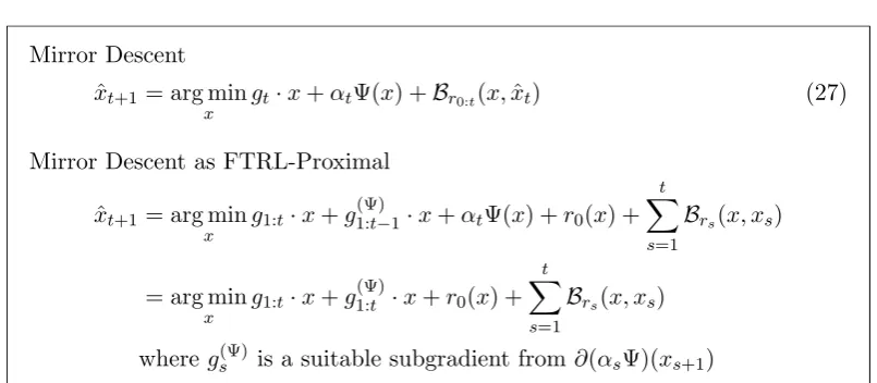
gt·x+αtΨ(x) +Br0:t(x,xˆt). (27)
We use ˆxto distinguish this update from an FTRL update we will introduce shortly. Building on the previous section, we allow the update to include an additional regu-larization termαtΨ(x). As before, typicallygt·x should be viewed as a subgradient approximation to a loss function `t; it will become clear that a key question is to what extent Ψ is also linearized.
Mirror Descent algorithms were introduced in Nemirovsky and Yudin (1983) for the optimization of a fixed non-smooth convex function, and generalized to Bregman divergences by Beck and Teboulle (2003). Bounds for the online case appeared in Warmuth and Jagota (1997); a general treatment in the online case for composite objectives (with a non-adaptive learning rate) is given by Duchi et al. (2010b). Following this existing literature, we might term the update of Eq. (27) Adaptive Composite-Objective Online Mirror Descent; for simplicity we simply refer to Mirror Descent in this work.
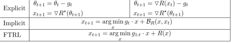
4. In particular, it is common to see updates written in terms ofOr?(θ) for a strongly convex regu-larizerr, based on the fact thatOr?(−θ) = arg minxθ·x+r(x) (see Lemma 15 in Appendix B). 5. Certain properties of Bregman divergences require φ to be strictly convex, but it provides a
Implicit updates For the moment, we neglect the Ψ terms and consider convex per-round losses `t. While standard Online Gradient Descent (or Mirror Descent) linearizes the `t to arrive at the update ˆxt+1= arg minx gt·xt+Br0:t(x,xˆt), we can
define the alternative update
ˆ
xt+1= arg min x
`t(x) +Br0:t(x,xˆt), (28)
where we avoid linearizing the loss`t. This is often referred to as an implicit update, since for general convex `t it is no longer possible to solve for ˆxt+1 in closed form. The implicit update was introduced by Kivinen and Warmuth (1997), and has more recently been studied by Kulis and Bartlett (2010).
Again considering the Ψ terms, the Mirror Descent update of Eq. (27) can be viewed as a partial implicit update: if the real loss per round is `t(x) +αtΨ(x), we linearize the `t(x) term but not the Ψ(x) term, taking ft(x) =gt·x+αtΨ(x). Generally this is done for computational reasons, as for common choices of Ψ such as Ψ(x) = kxk1 or Ψ(x) = IX(x), the update can still be solved in closed form (or at least in a computationally efficient manner, e.g., by projection). However, while αtΨ is handled without linearization, we shall see that echoes of the past α1:t−1Ψ are encoded in a linearized fashion in the current state ˆxt.
On terminology In the unprojected and non-adaptive case, the Mirror Descent update ˆxt+1 = arg minxgt·x+Br(x,xˆt) is equivalent to the FTRL updatext+1 = arg minxg1:t·x+r(x) (see Appendix C). In fact, Shalev-Shwartz (2012, Sec. 2.6) refers to this update (with linearized losses) explicitly as Mirror Descent.
In our view, the key property that distinguishes Mirror Descent from FTRL is that for Mirror Descent, the state of the algorithm is exactly ˆxt ∈Rn, the current
feasible point. For FTRL on the other hand, the state is a different vector in Rn,
for example g1:t for Dual Averaging. The indirectness of the FTRL representation makes it more flexible, since for example multiple values of g1:t can all map to the same coefficient value xt.
6.1 Mirror Descent is an FTRL-Proximal Algorithm
We will show that the Mirror Descent update of Eq. (27) can be expressed as the FTRL-Proximal update given in Figure 2. In particular, consider a Mirror Descent algorithm defined by the choice ofrt fort≥0. Then, we define the FTRL-Proximal update
xt+1 = arg min x
Mirror Descent
ˆ
xt+1= arg min x
gt·x+αtΨ(x) +Br0:t(x,xˆt) (27)
Mirror Descent as FTRL-Proximal
ˆ
xt+1= arg min x
g1:t·x+g1:(Ψ)t−1·x+αtΨ(x) +r0(x) + t
X
s=1
Brs(x, xs)
= arg min x
g1:t·x+g1:(Ψ)t ·x+r0(x) + t
X
s=1
Brs(x, xs)
whereg(Ψ)s is a suitable subgradient from ∂(αsΨ)(xs+1)
Figure 2: Mirror Descent as normally presented, and expressed as an equivalent FTRL-Proximal update.
for an appropriate choice g(Ψ)t ∈∂(αtΨ)(xt+1) (given below), where rtB is an incre-mental proximal regularizer defined in terms ofrt, namely
r0B(x)≡r0(x)
rtB(x)≡ Brt(x, xt) =rt(x)− rt(xt) +Ort(xt)·(x−xt)
fort≥1.
Note that rtB is indeed minimized by xt and rBt(xt) = 0. We require g(Ψ)t ∈ ∂(αtΨ)(xt+1) such that
g1:t+g(Ψ)1:t +Or B
0:t(xt+1) = 0. (30)
The dependence of g(Ψ)t on xt+1 is not problematic, as gt(Ψ) is not necessary to computext+1 using Eq. (29). To see (inductively) that we can always find a a g
(Ψ) t satisfying Eq. (30), note the subdifferential of the objective of Eq. (29) atx is
g1:t+g(Ψ)1:t−1+∂(αtΨ)(x) +Or0:Bt(x). (31) Since xt+1 is a minimizer, we know 0 is a subgradient, which implies there must be a subgradient gt(Ψ) ∈ ∂(αtΨ)(xt+1) that satisfies Eq. (30). The fact we use a subgradient of Ψ atxt+1rather thanxtis a consequence of the fact we are replicating the behavior of a (partial) implicit update algorithm.
Finally, note the update
xt+1 = arg min x
g1:t·x+g1:(Ψ)t ·x+r B
is equivalent to Eq. (29), since Equations (30) and (31) imply 0 is in the subgradient of the objective Eq. (29) at the xt+1 given by Eq. (32). This update is exactly an FTRL-Proximal update on the functionsft(x) = (gt+g(Ψ)t )·x.
With these definitions in place, we can now state and prove the main result of this section, namely the equivalence of the two updates given in Figure 2:
Theorem 11 The Mirror Descent update of Eq. (27) and the FTRL-Proximal up-date of Eq. (29) select identical points.
ProofThe proof is by induction on the hypothesis that ˆxt=xt. This holds trivially fort= 1, so we proceed by assuming it holds fort.
First we consider the xt selected by the FTRL-Proximal algorithm of Eq. (29). Since xt minimizes this objective, zero must be a subgradient at xt. Letting gs(r) =
Ors(xs) and notingOrtB(x) =Ort(x)−Ort(xt), we haveg1:t−1+g(Ψ)1:t−1+Or0:t−1(xt)− g(0:rt)−1 = 0 following Eq. (31). Since xt = ˆxt by induction hypothesis, we can rear-range and conclude
−Or0:t−1(ˆxt) =g1:t−1+g1:(Ψ)t−1−g0:(rt)−1. (33) For Mirror Descent, the gradient of the objective in Eq. (27) must be zero for ˆxt+1, and so there exists a ˆgt(Ψ)∈∂(αtΨ)(ˆxt+1) such that
0 =gt+ ˆg(Ψ)t +Or0:t(ˆxt+1)−Or0:t(ˆxt)
=gt+ ˆg(Ψ)t +Or0:t(ˆxt+1)−Or0:t−1(ˆxt)−g(tr) IH andOrt(xt) =g(tr) =gt+ ˆg(Ψ)t +Or0:t(ˆxt+1) +g1:t−1+g(Ψ)1:t−1−g
(r) 0:t−1−g
(r)
t Using Eq. (33)
=g1:t+g1:(Ψ)t−1+ ˆg (Ψ)
t +Or0:t(ˆxt+1)−g(0:rt) =g1:t+g1:(Ψ)t−1+ ˆg
(Ψ) t +Or
B
0:t(ˆxt+1).
The last line implies zero is a subgradient of the objective of Eq. (29) at ˆxt+1, and so ˆxt+1 is a minimizer. Since r0:t is strongly convex, this solution is unique and so ˆ
xt+1 =xt+1.
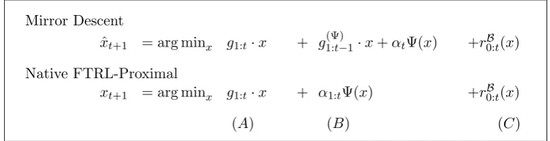
6.2 Comparing Mirror Descent to the Native FTRL-Proximal Algorithm, and the Application to L1 Regularization
Mirror Descent ˆ
xt+1 = arg minx g1:t·x + g (Ψ)
1:t−1·x+αtΨ(x) +rB0:t(x) Native FTRL-Proximal
xt+1 = arg minx g1:t·x + α1:tΨ(x) +rB0:t(x)
(A) (B) (C)
Figure 3: Mirror Descent expressed as an FTRL-Proximal algorithm compared to the Native FTRL-Proximal algorithm.
Both algorithms use a linear approximation to the loss functions `t, as seen in column (A) of Figure 3, and the same proximal regularization terms (C). The key difference is in how the non-smooth terms Ψ are handled: Mirror Descent approxi-mates the past αsΨ(x) terms for s < t using a subgradient approximation gs(Ψ)·x, keeping only the currentαtΨ(x) term explicitly. In Native FTRL-Proximal, on the other hand, we represent the full weight of the Ψ terms exactly asα1:tΨ(x). That is, Mirror Descent is applying significantly more linearization than Native FTRL-Proximal.
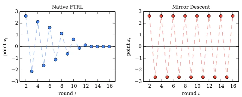
Why does this matter? As we will see in Section 6.3, there is no difference in the regret bounds, even though intuitively avoiding unnecessary linearization should be preferable. However, there can be a substantial practical differences for some choices of Ψ. In particular, we focus on the common and practically important case of L1 regularization, where we take Ψ(x) =kxk1. Such regularization terms are often used to produce sparse solutions (xtwhere manyxt,i = 0). Models with few non-zeros can be stored, transmitted, and evaluated much more cheaply than the corresponding dense models.
As discussed in McMahan (2011), it is precisely the explicit representation of the fullα1:tkxk1 terms that lets Native FTRL produce much sparser solutions when compared with the composite-objective Mirror Descent update withL1 regulariza-tion (equivalent to the FOBOS algorithm of Duchi and Singer (2009)). This argu-ment also applies to Regularized Dual Averaging (RDA, a Native FTRL-Centered algorithm); Xiao (2009) presents experiments showing the advantages of RDA for producing sparse solutions. In the remainder of this section, we explore the appli-cation to L1 regularization in more detail, in order to illustrate the effect of the additional linearization of the kxk1 terms used by Mirror Descent as compared to the Native FTRL-Proximal algorithm.