Volume 2, Issue 10, October 2013
Page 330
Abstract
In this paper Design of Experiments for turning the austenitic AISI 302 material for prediction of Tool life, surface Roughness and cutting force are taken in to consideration as output parameters for these experiments. Process parameters (cutting speed, feed rate, depth of cut and tool nose radius) are used as inputs for indentifying the machinability of the material. Response Surface Regression method is used for prediction of machinability of the material by using this experimental data.
Key Words: AISI 302, Surface Roughness, Design of Experiments (DOE).
1. Introduction
Predicting process of machinability models and determining the optimum values of process parameters in manufacturing systems have been areas of interest for researchers and manufacturing engineers. Machinability database systems are essential for selecting optimum process parameters during the process planning stage which represents an important component in Computer Integrated Manufacturing (CIM) [1]. Most of these researchers have used the generalized empirical equations systems that utilize expanded Taylor tool life equations to determine proper machining conditions based on three criteria: minimum production cost, maximum production rate or maximum profit rate per item. These criteria have been considered in both constrained and unconstrained problems of machining economics. Tool life, surface roughness and cutting forces have an effect on cost, time, design features and quality of manufacturing operations. In addition, these machinability models are very critical constraints for process parameters selection in process planning systems. Therefore, accurate representation of these three important factors in empirical models is very important. These models cannot be predicted without experimental work on specific material using specific conditions.
A considerable amount of studies have investigated the general effects of process parameters (cutting speed, feed rate, depth of cut, etc.) on process functions (tool life, cutting force and surface roughness) [1,3]. Most of these models are based on RA, very few papers used CNN [4–9].
2. Experimental Setup
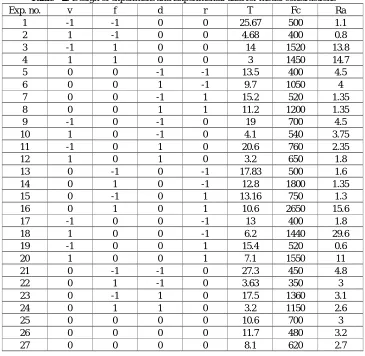
The obtained machinability models are compared against each other using the relative error analysis, descriptive statistics and hypothesis testing. Four machining parameters were considered (cutting speed (v, m/min), feed rate (f, mm/r), depth of cut (d, mm) and tool nose radius (r, mm)). considered four machining parameters (cutting speed (v, m/min), feed rate (f, mm/r), depth of cut (d, mm) and tool nose radius (r, mm)). The considered outputs are tool life (T, min), cutting force (Fc, N) and surface finish (Ra, _m). The four process parameters were considered at three levels (−1, 0 and 1) as shown in Table 1. The experiments are conducted based on Box and Dehnken design. This design is rotatable and consists of blocks in an orthogonal arrangement. This inputs and responses are illustrated in Table 2.
Table - 1: Factors and levels of the experiment for model constructions
Level
Factors
Cutting Speed (v) m/min
Feed (f) mm/rev
Depth of Cut (d)
mm Nose Radius (r) mm
level (-1) 25 0.1 0.25 0.4
level (0) 60 0.25 0.5 0.8
level (1) 144 0.7 1.6 1.6
PREDICTIVE MACHINABILITY MODEL OF
HARDENED STEEL MATERIAL IN
TURNING OPERATION BY RESPONSE
SURFACE REGRESSION METHOD
Manu Ravuri1, Akbar Basha.S2, Sharmas Vali.S3
1,2,3 Assistant Professor, Department of Mechanical Engineering,
Volume 2, Issue 10, October 2013
Page 331
3. Results
Table - 2: Design of experiment and Experimental data for model constructions
Exp. no. v f d r T Fc Ra
1 -1 -1 0 0 25.67 500 1.1
2 1 -1 0 0 4.68 400 0.8
3 -1 1 0 0 14 1520 13.8
4 1 1 0 0 3 1450 14.7
5 0 0 -1 -1 13.5 400 4.5
6 0 0 1 -1 9.7 1050 4
7 0 0 -1 1 15.2 520 1.35
8 0 0 1 1 11.2 1200 1.35
9 -1 0 -1 0 19 700 4.5
10 1 0 -1 0 4.1 540 3.75
11 -1 0 1 0 20.6 760 2.35
12 1 0 1 0 3.2 650 1.8
13 0 -1 0 -1 17.83 500 1.6
14 0 1 0 -1 12.8 1800 1.35
15 0 -1 0 1 13.16 750 1.3
16 0 1 0 1 10.6 2650 15.6
17 -1 0 0 -1 13 400 1.8
18 1 0 0 -1 6.2 1440 29.6
19 -1 0 0 1 15.4 520 0.6
20 1 0 0 1 7.1 1550 11
21 0 -1 -1 0 27.3 450 4.8
22 0 1 -1 0 3.63 350 3
23 0 -1 1 0 17.5 1360 3.1
24 0 1 1 0 3.2 1150 2.6
25 0 0 0 0 10.6 700 3
26 0 0 0 0 11.7 480 3.2
27 0 0 0 0 8.1 620 2.7
3.1 Response surface method
Response surface methods are used to examine the relationship between one or more response variables and a set of quantitative experimental variables or factors. These methods are often employed after identifying the controllable factors and the objective is to find the factor settings that optimize the response. Designs of this type are usually chosen when there is suspecting curvature in the response surface. It is clear from the literature that the tool life, cutting force and surface finish equations are not linear and they could be predicted using the response surface method. The initial analysis of the output obtained from RSM includes all parameters and their interactions. The models are reduced by eliminating elements which have no significant effect on the responses. The revised RSM analysis is illustrated in Table
3.1.1. Response Surface Regression: Time versus A, B, C The analysis was done using coded units.
Estimated Regression Coefficients for Time
Term Coef SE Coef T P
Constant 11.3637 1.537 7.392 0
A -5.8392 1.031 -5.662 0
B -5.6858 1.031 -5.513 0
C -1.4442 1.031 -1.4 0.179
A*A -1.4597 1.458 -1.001 0.331
B*B 0.7178 1.458 0.492 0.629
C*C 1.2278 1.458 0.842 0.412
A*B 4.8275 1.786 2.703 0.015
A*C -0.625 1.786 -0.35 0.731
B*C 2.3425 1.786 1.311 0.207
Volume 2, Issue 10, October 2013
Page 332
Analysis of Variance for TimeSource DF Seq SS Adj SS Adj MS F P
Regression 9 971.77 971.77 107.974 8.46 0
Linear 3 822.12 822.12 274.041 21.47 0
Square 3 32.91 32.91 10.971 0.86 0.481
Interaction 3 116.73 116.73 38.91 3.05 0.057
Residual Error 17 216.97 216.97 12.763
Lack-of-Fit 9 190.98 190.98 21.22 6.53 0.007
Pure Error 8 25.99 25.99 3.248
Total 26 1188.73
3.1.2. Response Surface Regression: Fc versus A, B, C The analysis was done using coded units.
Estimated Regression Coefficients for Fc
Term Coef SE Coef T P
Constant 957.41 215.6 4.44 0
A 229.17 144.7 1.584 0.132
B 320 144.7 2.212 0.041
C 267.5 144.7 1.849 0.082
A
A -165.69 204.6 -0.81 0.429B
B 140.56 204.6 0.687 0.501C
C -188.19 204.6 -0.92 0.37A
B 287.5 250.5 1.148 0.267A
C 12.5 250.5 0.05 0.961B
C -27.5 250.5 -0.11 0.914S = 501.1 R-Sq = 46.1% R-Sq(adj) = 17.6%
Analysis of Variance for Fc
Source DF Seq SS Adj SS Adj MS F
Regression 9 3652298 3652298 405811 1.62 0.188
Linear 3 2717683 2717683 905894 3.61 0.035
Square 3 600340 600340 200113 0.8 0.512
Interaction 3 334275 334275 111425 0.44 0.725
Residual Error 17 4268420 4268420 251084
Lack-of-Fit 9 3819420 3819420 424380 7.56 0.005
Pure Error 8 449000 449000 56125
Total 26 7920719
3.1.3. Response Surface Regression: Ra versus A, B, C The analysis was done using coded units.
Estimated Regression Coefficients for Ra
Term Coef SE Coef T P
Constant 5.52963 2.619 2.111 0.05
A 4.20833 1.757 2.395 0.028
Volume 2, Issue 10, October 2013
Page 333
C -0.5583 1.757 -0.318 0.755
A
A 1.76597 2.485 0.711 0.487B
B -0.9903 2.485 -0.399 0.695C
C -2.6965 2.485 -1.085 0.293A
B 3.55 3.043 1.167 0.259A
C 0.05 3.043 0.016 0.987B
C 0.325 3.043 0.107 0.916S = 6.086 R-Sq = 39.2% R-Sq(adj) = 7.1% Analysis of Variance for Ra
Source DF Seq SS Adj SS Adj MS F P
Regression 9 406.7 406.7 45.19 1.22 0.345
Linear 3 269.81 269.81 89.94 2.43 0.101
Square 3 86.05 86.05 28.68 0.77 0.524
Interaction 3 50.84 50.84 16.95 0.46 0.715
Residual Error 17 629.65 629.65 37.04
Lack-of-Fit 9 345.77 345.77 38.42 1.08 0.461
Pure Error 8 283.88 283.88 35.48
Total 26 1036.35
From the above table the empirical models of the tool life, cutting force and surface finish are as follows
Time (t) = 11.36337-5.83917xA – 5.68583 x B – 1.44417 x C – 1.45972 x A2 + 0.717778 X B2+ 1.22778 x C2 + 4.82750 x A x B – 0.625000 x A x C + 2.34250 x B x C
Cutting Force (Fc) = 957.407 229.167 A+320.000 B+267.500 C-165.694 A2+140.556 B2-188.194 C2 +287.500 A B+12.5000 A C-27.5000 B C
Surface Roughness (Ra) = 5.52963+4.20833 A+2.11250 B -0.558333 C+1.76597A2 -0.990278 B2-2.69653 C2+3.55000 A B+ 0.0500000 A C+0.325000 B C
4. Conclusion
In this paper, empirical data for prediction of machinability model (tool life, cutting force and surface roughness) have been developed based on response surface methodology. The developed machinability model can be utilized to formulate an optimization model for the machining economic problem to determine the optimal values of process parameters for the selected material.
References
[1] I. Coudhury, M. El-Baradie, Machinability assessment of inconel 718 by factorial design of experiment coupled with response surface methodology, J. Mater. Process. Technol. 95 (1999) 30–39.
[2] K. Taraman, Utilization of design of experiments for reduced cost and added reliability, SME (1981).
[3] L. Ozler,A. Ozel, Theoretical and experimental determination of tool life in hot machining of austenitic manganese steel, Int. J. Mach. Tool Manufact. 41 (2001) 163–172.
[4] U. Zuperl, F. Cus, B. Mursec, T. Ploj, A hybrid analytical-neural network approach to the determination of optimal cutting conditions, J. Mater. Process. Technol. 175 (2004) 82–90.
[5] S. Wong, A. Hamouda, Machinability data representation with artificial neural network, J. Mater. Process. Technol. 138 (2003) 538–544.
[6] N. Tosum, L. Ozler, A study of tool life in hot machining using artificial neural networks and regression analysis method, J. Mater. Process.Technol. 124 (2002) 99–104.
[7] C. Feng, X.Wang, Digitizing uncertainty modeling for reverse engineering applications: regression vs. neural networks, J. Intell. Manufact. 13 (2002) 189–199.
[8] T. Ozel,Y. Karpat, Predictive modelling of surface roughness and tool wear in hard turning using regression and neural networks, Int. J. Mach. Tool Manufact. 45 (2005) 467–479.
Volume 2, Issue 10, October 2013
Page 334
AUTHORS
Manu Ravuri received the B.Tech in Mechanical Engineering from Dr. Paul Raj Engineering Collage, Bhadarachalam in year 2008, and received Masters Degree in Manufacturing Engineering form National Institute of Technology Karanataka, Surathkal in the year 2012, he is staying in Madanapalle and working as Assistant Professor in Department of Mechanical Engineering at Madanapalle Institute of Technology & Science, Madanapalle. Have many International and National Journals and attended many conferences and workshops, editorial board Reviewer for International Journal of Technology Enhancements and Emerging Engineering Research (IJTEEE).
Sharmas vali.S received the B.Tech in Mechanical Engineering from MITS, Madanapalle in year 2007, and received Masters Degree in R&AC form JNTUA, Anatapur in the year 2011, he staying in Madanapalle and working as Assistant Professor in Department of Mechanical Engineering at Madanapalle Institute of Technology & Science, Madanapalle. Have many International and National Journals and attended many conferences and workshops.