A fast adaptive neural network system for intelligent control

MURDOCH RESEARCH REPOSITORY

http://dx.doi.org/10.1109/ICSMC.1997.638082

Zaknich, A. and Attikiouzel, Y. (1997) A fast adaptive neural

network system for intelligent control. In: IEEE International

Conference on Systems, Man, and Cybernetics, Computational

Cybernetics and Simulation, 12 - 15 October, Orlando, FL, USA,

1023 - 1027 vol.2.

http://researchrepository.murdoch.edu.au/20136/

Copyright © 1997 IEEE

Personal use of this material is permitted. However, permission to reprint/republish

this material for advertising or promotional purposes or for creating new collective

A Fast Adaptive Neural Network System for Intelligent Control

Anthony Z h c h , Member

IEEE, Associate Member

AES

Yianni Attikiouzel.

Fellow

IEEE.

Fellow

IEE,

Fellow

IEAust

Centre for Intelligent Information Processing Systems (CIIPS), Department of Electrical and Electronic Engineering,

The University of Western Australia, Nedlands 6907, Western Australia. Email: [email protected]

ABSTRACT

An intelligent control system needs to adapt to new dynamics very quickly but also retain knowledge of past dynamics to be able to act effectively and quickly for repeat occurrences. One solution is to model the system with two neural networks in parallel whereby one network is trained a priori with a wide range of historical dynamics while the second one, is allowed to adapt itself to make up the differences between the first model and the real-time dynamics. Within this scheme, as the second network is called to adapt itself, the first one can be progressively trained to learn the new dynamics without adversely affecting the old training. A

strategy of this type can be achleved very effectively using the Modified Probabilistic Neural Network because it is constructed with local radial kernel functions and its adaptation mechanism is computationally simple and very fast. This is demonstrated using a complex nonlinear system whose characteristics suddenly change after initial training and then switch back to the original characteristics. Comparisons are made with other networks to show the important advantages of the Modified Probabilistic Neural Network.

1.0 INTRODUCTION

An adaptive network can be used to model either a lincar system whose parameters are unknown (or changing with time) or a nonlinear system whose model is unknown (or also changing with time). A

linear adaptive system will eventually converge to a linear solution over sufficient time and range of input signals. It will continue to adapt, only if the system or noise statistics change. For a nonlinear system, a linear adaptive system can only adapt to a linear approsimation at the current operating point. It is possible however, to keep a historical record of the set of linear models for each small region around a set of operating points and then apply an appropriate model as

the set point changes. This is called schedule or switching control with multiple models. A nonlinear adaptive network ~1.111 adapt to a more accurate model at the current operating point. but like the linear adaptive network it cannot generalise tius to new operating

points, unless a historical record is kept. To ensure a more robust control of nonlinear systems it is desirable to have some historical information about the system over the expected range of operating points in parallel with a fast adaptive network to make up any Merences.

In references (1.21 it is shown how a Neural Network

0

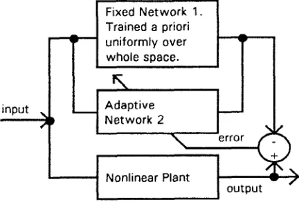
structure as depicted in Figure 1 can be used to model a plant's nonlinear dynamic behaviour when certain information is known a priori and the remaining information needs to be learned. Neural Network 1 is trained to learn the plant's known dynamic behaviour whereas Neural Network 2 is used to learn on-line the initially unknown behaviour. Of course once the new behaviour occurs it would be sensible to accumulate the data and include it as history in the a priori model represented by Network 1. If the system is not changing continually into new operating modes then eventually Network 2 will become superfluous and operation can be effected through Network 1.

Fixed Network 1.

Trained a priori uniformly over whole space.

input

4

Adaptive

Network 2

I

Nonlinear Plant

I

I

output

-

Figure 1. Nonlinear Forward Modelling Scheme

A single Modified Probabilistic Neural Network (MPNN) [3,4] can be used to replace the two neural networks in Figure 1 and still achieve similar functionality. This can be done because the MPNN is based on a set of radial basis functions which provide the property of localised influence. This allows the learning system to develop and refine its control very

quickly in one region of the measurement space without affecting its learning in distant regions. The MPNN is initially trained with all available a priori data and then it systematically integrates all new data as it begins to operate. This is demonstrated with an illustrative example of modelling a complex recursive nonlinear plant. The MPNN is compared with a Multi-Layer Perceptron (MLP) to show the practical benefits, including faster adaptation, better retention of past learning, and better ability to deal with variable system noise. The MPNN architecture and adaptation schemes are reviewed in the next two sections followed by the illustrative example and conclusions.

2.0 REVIEW OF THE MODIFIED PROBABILISTIC NEURAL NETWORK

The Modified Probabilistic Neural Network (MPNN) was initially introduced by Zaknich et al in 1991 [3]. It is closely related to Specht's General Regression Neural Network (GRNN) [SI and both are related to Specht's Probabilistic Neural Network (P") classifier. The method of the basic MPNN/GR" has similarities with the method of Moody and Darken [ 6 ] ; the method of radial basis functions [7]; and a number of other nonparametric kernel based regression techniques stemming from the work of Nadaraya [SI and Watson

[9].

If

it can be assumed that for each local region in the input space, represented by a centre vector ci, there is a corresponding scalar output yi that it m p s into, then the general model to use for all forms of the

MPNN and even the GRNN is equation (1).

i=l

ci centre vector for class i in the input space. 0 learning parameter chosen during training. yi output related to ci (real valued or quantised). M number of unique centres ci.

Zi number of vectors xj associated with centre ci. NS total number of training vectors (Sum of Zi ).

h&)

is a radial basis function.

A Gaussian radial basis function is often used for

A&)

as defined in equation (2) but there are many other suitable radial basis functions which can be chosen in place of the Gaussian function. All the radial basis functions have exactly the same learning parameter G chosen during training.

-(x-ci) T ( x - c i )

20-2 ( 2 )

r;.

(XI = exp

Equation (1) represents the G R " if all the Z;= 1, the yi are real valued, the centre vectors ci are replaced with individual training vectors xi and M=NS. The MPNN can be seen as a kind of s u e reduced G R " as it has virtually the same performance specifications as the GRNN, but in a more computationally efficient structure. There are many ways to select of the parameters M,

Z

i

and ci for the MPNN but in all cases the selection is done vely simply with minimal computational requirements [4, lo].

3.0 MPNNlGR" ADAPTATION SCHEME

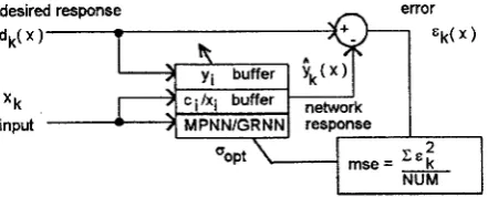
The basic adaptive structure for the MPNN/GR" is depicted in Figure 2 . The actual input and desired data are fed directly into the MPNN/GR" storage buffers to be used in the network architecture. In the case of the G R " the data {xi+yi

I

i=1,

...

NS} are used without any modification, but in the case of MPNN they are reduced with minimal computational complexity [4,10] to {ci+yi

I

i=1,

...

M}

before storage. Adaptation involves finding the optimal G giving the minimum mse for some fixed number NUM of known sample vectors passing through the network. For most problems the ( m e vs a) curve is smooth with a single minimum and it easy to find a suitable G.

desired response

-

error

I

'k

inout _{I 1}

-x a ;

m e =

-

=opt

\

NUM

Figure 2. Basic MPNN/GR" Adaptive Structure

In the case of the G R " the training data simply flows through a fixed sized delay line buffer so that old data are lost as new data come in. This ensures fast system adaptation to changing statistics because the network is constructed from data of the recent past only. In the case of the MPNN for a new data pair {x + yi}, categorised

as belonging to the centre i, it adds to the training data according to equations (3) and (4)

Zl"=

z y + 1

(3)

only if new training vector x belongs to ci.

if Zi > 0 and new training vector x belongs to ci, else

if Zi = 0, cVew = x , the associated yi is also added.

1

Thc new vector pair { x

+

y,} is deemed to belong to the class i if thc quantised characterisation vector niadc from thc quantised elements of ( x

+

yi} matches the specific characterisation vector defining class i. The exact nature of that quantised characterisation vector depends on the characterisation Method A or B [lo] chosen. For Method A it only depends on the quantised output values whereas in Method B it includes both the input and output quantised vector elements.

Equations (3) and (4) are strictly only valid for stationary data statistics. Eventually, the centre vectors, cincw, will converge at which time the accumulation

may bc stopped or continued with no detrimental effects Onc way to solve this problem when Method B is used is to also check whether x belongs to the quantised input part of the characterisation vector. If it does, but the output part does not match, then reduce the corresponding Zi by 1; if Zi 2 1 create a new class. In this way old irrelevant training will eventually be extinguished and replaced uith new learning without afTecting any other learning in the network.

For changing statistics or for self regulation it is also possible to introduce a forgetting factor z expressed in ternis of a discrete number of update sample points into equations (3) and (4) as follows.

( 5 )

( z - 1 )

zpU+

1

z

zl""'

=

if new training vector x belongs to ci.

if new training vector

x

does not belong to ci.

( Z j

-

1 )

c y +

x

(7)

Zi C Y W =

if Zi > 0 and new training vector x belongs to ci, else if Zi =0, crew = x , the associated yi is also added.

While the buffers are being loaded as described above, CT

is adapted to maintain optimal performance. For stationary signal and noise statistics once the buffers are filled for the GRNN, or the centres have converged for the "N, and an optimum ooet has been established, it can then be fixed along with the buffer data. Otherwise, o must be periodically adapted as the data flows through the buffers.

as described below, where x(iii is the input and .v(n) is

the output sequence.

Initially the system output for state 1 is simply

y=y(rz+l). At some later time it suddenly changes to state 2: y=(j(n+l))2 for y(n+1)2Q and, v=-&(n+l))'

for y(n+l)'-O and then later in time switches back to the initial state 1. For each state the same inputs produce distinctly different outputs which provides an extreme case study.

Training and testing digital signal sequences of 500 points each were simulated according to equations (IO) and (1 1) respectively.

2 d

x ( n ) = sin(-) (10)

250

21dc 21dc

250 25

x ( n ) =0.8sin(-) +0.2sin(-) (11)

In addition to these signals a further 500 points of a random sequence bandlimited to 0-4.0 Hz (assuming a Nyquist sampling frequency of 100 Hz) €or training and another 500 independent points for testing, for each plant, were also simulated. These sequences along with their desired outputs are shown in Figures 3 and 4.

There were 1000 training and 1000 testing vector pairs for each of the two states.

The neural network input vector

x

was constructed according to equation (12) indicating a recursive design.

Given the training and testing vectors for state 1 a MLP

(5-20-1) with 20 hidden nodes, a GRNN with 1000 hidden nodes, a Method B Ml"N with 662 hidden nodes and input quantisation level N,=2 and output quantisation level N=4096 and a Method B MPNN with 149 hidden nodes and input quantisation level N,=2

and output quantisation level N=128 were trained a priori and the results are shown in Table I. The table shows the number of training iterations, the mean squared error (mse) between the outputs and desired outputs, the training and vector evaluation times for each network implemented in C and run on an IBM compatible PC Pentium 90. Table I also shows testing results when random noise with a uniform distribution and variance of 0.021 is added to the testing input

vectors.

4.0 AN ILLUSTRATIVE EXAMPLE

Equation (8) (Narendra and Parthasarathy's [ I l l type 4

1

0

-1

200 4m Mx) Bw lD00

salelaM2wningilpAseqwmze

GRNN

5-1000-1

MPNN MethB

1 . n . ?

noisy

train 1 tcst

noisy

eain 1

test

Y . I

200 4m Mx) Bw lD00

-1 '

salelaM2wningilpAseqwmze

Net.

Type

MLP

5-20-1

G R "

5-1Ooo-1 MPNN Meth.B 5-548-1 Nx=2 N=4096 MPNN

Met h B

I

O

-1

0 m 400 600 800 loo0

Statblte~dsstndaUau(

1 , I

Data Set eain test noisy tram noisy train test noisy test train test I

2W 400 Mw) Mw) 1wO

Stale 2 bnining cbsired ouipui

Figure 3. Training sequences

1

0

I,

1 _I

0

-1

0 m 400 600 800

State 2teshgdesid cupd

Figure 4. Testing sequences

If the parallel setup of Figure 1 is adopted with network 1 trained a priori for state 1 Network 2 adaptively learns the difference between state 1 and state 2 as state 2

training data begins to occur. Then network unlearns it when state 1 data is reintroduced. The training times shown in Tables I and 11 are typical of the times required for Network 2 to adapt itself either way and they represent the extreme case of adapting to distinctly different dynamics. The MPNN/GR" methods adapt to their optimal points after exactly 1000 new points which represents the total number of training points for each state. The MLP on the other hand takes considerably longer in terms of both training time and number of training iterations. The MLP used simple gradient descent learning (gain factor of 0.01 and momentum factor of 0.001) which is the slowest learning method. However, whatever method is adopted it will never learn faster than the MPNN/GRNN which simply takes the new training data a point at a time and systematically adds it to its structure according to adaptation equations (3) and (4) or equations ( 5 ) , (6)

and (7).

Instead of using the parallel setup of 1 a single MPNN

can be used in conjunction with adaptation equations (3)

and (4) plus the extra processing suggested for Method

B.

This would achieve exactly the same results as shown

in Tables I and 11. This approach offers considerable advantage for intelligent control applications. New dynamics are integrated and retained in the structure and are not extinguished except in the specific case when they should be replaced to avoid erroneous operation. Any changes only al€ect local regions in the operating space leaving historical data in other regions in tact. With only v e y minor modifications it is also possible to build a system similar to schedule or switching control with multiple models by idenUfylng separate regions of the MPNN space which have been trained with specific dynamics. An identification vector according to equation (13) can i d e n w the Merent dynamic states and activate the respective region of the MF"N space.

Tnin

itsrJ

passes

400.o0o

I Meth.B

I

test

I

rABLE I

men

I

U

I

Train

1

VerL

I

0.00012

I

-

132.4

in sec

0.00033

0.00972

0.00314

I

0.135

I

I ~ I 6.32 I

0.00024

I

0.029

I

I

0.00632 0.00357 0.111

I

Training results for state 2 are shown in Table 11.

TABLE IT

iter./

1300000 0.00016

0.00153 0.108

U

1

I

O.&SI

I

O.&

1

1.10

Vect. evd.

in Sec

0.00033

0.00972

0.00423

0.001 IO

5.0 CONCLUSIONS

It has been shown how the MPNN is very suitable for intelligent control applications. It has extremely fast adaptation abili6, the ability to absorb new local learning without adversely affecting previous global learning and v e v good noise tolerance. The MPNN is a general regression method which can be implemented in a simple parallel hardware structure.

6.0 REFERENCES

Warwick, K., Irwin, G. W. and Hunt, K. J., editors for "Neural networks for control and systems", Peter Pengrinis. London. 1992.

Mller, W. T.., Sutton, R. S. and Werbos, P. J., "Neural networks for control", MIT Press, MA, 1990.

Zaknich, Anthony, desilva, Christopher and Attikiouzel, Yianni, "The probabilistic neural network for nonlinear time series analysis", IEEE International Joint Conference on Neural Networks (IJCNN), Singapore, 17-2lSt November 1991, pp.

Zaknich. Anthony and Attikiouzel, Yianni, "Time series characterisation schemes for the modified probabilistic neural network", Australian Journal of Intelligent Information Processing Systems

(AJIIPS), Vol. 2, No. 2, Winter 1995, pp. 1-11.

Specht,

D.

F., "A general regression neural network", IEEE Transactions on Neural Networks, Vol. 2, No. 6, November 1991, pp. 568-576. Moody, J. and Darken, C., "Fast learning in networks of locally-tuned processing units", Neural Computation, Vol. 1 No. 2, September 1989, pp.

Powell, M. J. D., "Radial basis functions for multivariate interpolation:

A

review", Technical Report DAMPT 1985NA12, Department of Applied Mathematics and Theoretical Physics, Cambridge University, England, 1985.

Nadaraya, E. A., "On estimating regression", Theory Probab. Appl., 9, 1964, pp. 141-142. Watson, G. S . , "Smooth regression analysis", Sankhya Ser. A, 26, 1964, pp. 359-372.

1530-1535.

28 1-294.

[IOjZaknich, Anthony and Attikiouzel, Yianni, "A

modified probabilistic neural network signal processor for nonlinear signals", Proceedings of the 13th International Conference on Digital Si al

July, 1997.

[ I l l Narendra, K. S.. and Parthasarathy, K., "Identifcation and control of dynamical systems using neural networks", IEEE Transactions on Neural Networks, Vol. 1, March 1990, pp. 4-27. Processing @SP-97), Santorini, Greece, 2"

(Ig"

-4*