Design and Implementation of Digital Linear Control
Systems on Reconfigurable Hardware
Marcus Bednara
Department of Computer Sciences 12, Hardware-Software-Co-Design, Friedrich-Alexander-Universit¨at Erlangen, D-91058 Erlangen, Germany
Email:[email protected] Klaus Danne
Heinz Nixdorf Institute, University of Paderborn, D-33102 Paderborn, Germany Email:[email protected]
Markus Deppe
Mechatronic Laboratory Paderborn (MLaP), University of Paderborn, D-33098 Paderborn, Germany Email:[email protected]
Oliver Oberschelp
Mechatronic Laboratory Paderborn (MLaP), University of Paderborn, D-33098 Paderborn, Germany Email:[email protected]
Frank Slomka
Department of Computer Science, Embedded Hardware/Software Systems Group, Carl von Ossietzky Universit¨at Oldenburg, D-26111 Oldenburg, Germany
Email:[email protected] J ¨urgen Teich
Department of Computer Sciences 12, Hardware-Software-Co-Design, Friedrich-Alexander-Universit¨at Erlangen, D-91058 Erlangen, Germany
Email:[email protected]
Received 14 March 2002 and in revised form 15 October 2002
The implementation of large linear control systems requires a high amount of digital signal processing. Here, we show that re-configurable hardware allows the design of fast yet flexible control systems. After discussing the basic concepts for the design and implementation of digital controllers for mechatronic systems, a new general and automated design flow starting from a system of differential equations to application-specific hardware implementation is presented. The advances of reconfigurable hardware as a target technology for linear controllers is discussed. In a case study, we compare the new hardware approach for implementing linear controllers with a software implementation.
Keywords and phrases:digital linear control, reconfigurable hardware, mechatronic systems.
1. INTRODUCTION
Modern controller design methods try to support the de-sign of controllers at least semiautomatically. The need for a transparent and straightforward design process often leads to software implementations of controllers, that is, micro-processor programs specified in a high-level language using floating-point arithmetic. This approach, however, is
prototyping of complex linear control systems becomes pos-sible. Low-cost FPGA will allow their use in the final product in the near future. To support the use of hardware imple-mentations, however, new automated design flow methods are required.
The advances in silicon technology and the high compu-tational power of modern microprocessors and DSPs allow for implementation of flexible linear controllers in software. However, the implementation of state-space controllers for applications with high sample rates requires short computa-tional times. As the number of required calculations grows nonlinearly with the number of states, application-specific hardware is often unavoidable to provide sufficient compu-tational power. Yet dedicated hardware is very inflexible since it is impossible to adapt the implementation on changing re-quirements, new applications, or modified parameters. Re-configurable hardware structures provide a way out of this dilemma. With reconfigurable hardware, it is possible to de-sign an application-specific hardware along with the high flexibility of software solutions. For linear controllers, par-allelism can be used as needed and the implementation can be changed if required.
In this paper, we describe an approach for an automated mapping of linear controllers to reconfigurable hardware. Furthermore, we quantitatively compare such solutions to software implementations. We develop a generic hardware structure which can be easily adapted to new applications. In difference to [4], where a special instruction set processor for implementing digital control algorithms is described, our approach implements all parts of the controller in hardware. Important issues for using reconfigurable hardware are:
(1) What speedup can be obtained by the use of hardware as compared to a pure software solution?
(2) Do typical control systems fit current FPGA devices?
As a case study, we have implemented a linear controller for an inverse pendulum in hardware and software on an FPGA-based reconfigurable hardware platform and have compared the results. The experiments show the potential of recon-figurable hardware to implement fast and flexible solutions of linear control systems. Compared to pure software solu-tions which can also change the controller parameters during runtime, the new approach [5] has several advantages.
(1) The obtainable sample period only scales linearly with the problem size which allows for controller imple-mentations with very high sample rates.
(2) FPGAs offer the same flexibility as software implemen-tations along with the speed of application-specific hardware.
(3) If the applications require higher clock rates as sup-ported by the used FPGA technology, it is very easy to adapt the designed hardware to other faster silicon technologies such as gate arrays.
(4) By implementing different controllers in parallel for the same application, it could become very easy to switch between the controllers to adapt the sys-tem to changing-environmental parameters. By proper
w M
Prefilter
u
x0
x
−C
y
−R uR
Plant
Controller
Measurement equation ˙
x=A x+B u
A: System matrix
B: Input matrix
C: Output matrix
y: Plant output
x: State vector
u: Inputs
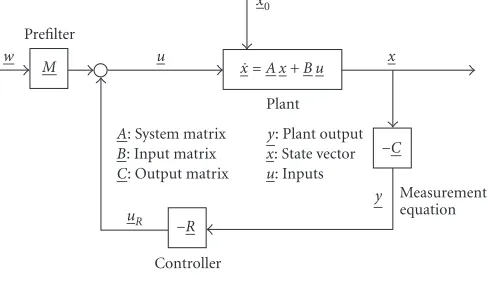
Figure1: General structure of a control system.
blending mechanisms, the controller will not remain in an undefined state during switching.
Especially the last item will be the subject of our future work. The paper is organized as follows. InSection 2, we give a basic overview of the mathematical principles of digital lin-ear control systems design. The design flow for the imple-mentation of linear systems of differential equations in re-configurable hardware is described inSection 3. A descrip-tion of the proposed architecture of the software and hard-ware implementation is given inSection 4.Section 5 intro-duces a case study on how linear controllers can be imple-mented on FPGAs and describes the complete design flow for the example. In this section, we also compare a soft-ware implementation of the example with the pure hardsoft-ware solution. We conclude with a discussion of future work in Section 6.
2. LINEAR CONTROLLERS
2.1. Structure
The basic idea of controlling a system (called control path or plant) is to take influence on its dynamic behavior via a con-trol feedback loop. A concon-troller takes measurements from the control path and computes new input variables to the sys-tem. This results in a typical feedback structure is shown in Figure 1. Generally, the system consisting of controller and control path is continuous, nonlinear, and time variant. In most cases, however, the controller and control path can be modeled as linear time-invariant systems (see Figure 1), where the plant is specified by a system of linear differential equations.
2.2. Mathematical foundations
w
A: System matrix
B: Input matrix
C: Output matrix
I: Identity matrix
L: Observer matrix
M: Prefilter matrix
R: Recoefficient matrix
u: Inputs
w: Command variable
x: States of plant
x0: States of plant ˆ
x: States of observer ˆ
xs: States of disturbance observer
y: Plant outputs
z: Disturbance
Figure2: Linear controller with state and disturbance observers.
is used to reconstruct the disturbance for a disturbance re-jection. The actual controller is a state vector feedback con-troller.Figure 2shows the generalized structure of the con-troller for the inverse pendulum that is used in the case study inSection 5. For our example, shown inSection 5, we do not need all the components of this structure. The implemented controller of the inverse pendulum consists of the state feed-back−Rand the observer which is necessary for reconstruct-ing the complete state vector. The disturbance feedforward component was not necessary for the example. In general, the whole controller (gray part ofFigure 2) can be expressed by a linear time-invariant state system ((1) and (2)).
The state-space approach is a unified method for model-ing and analyzmodel-ing linear time-invariant control systems. The equations are divided into two parts: a system of (1) relates the state variablesxand the input signalsu. A second sys-tem of (2) relates the state variablesxand the current input uto the output signalsy. The general form of the state-space equations is
˙
x=Ax+Bu, (1)
y=Cx+Du. (2)
Numerical processing
A common method for the realization of digital control sys-tems is now to (a) transform the differential equations into difference equations and (b) convert the variables and pa-rameters from the floating-point to fixed-point or integer numbers. The differential equations (1) and (2) are trans-formed into a system of recursive difference state equations (time discretization)
x(k+ 1)=Adx(k) +Bdu(k),
y(k)=Cdx(k) +Ddu(k).
(3)
Now the state and the output signals are represented by the sequences{x(k)}and{y(k)}.
Numerical integration methods like implicit rectangular or trapezoidal integration are thereby widely used to trans-form controllers from continuous time to discrete time. With an implicit rectangular integration method, the following equations represent the transformed matrices, whereTsis the discrete sample time andIis the identity matrix:
Ad=
When using implicit rectangular or trapezoidal integra-tion methods, we have to take into account that the matrices A,B,C, andDas well as the state vectorxare transformed (4). For scaling, the minimum and maximum values of x must be transformed as well:
xmax;minD =xmax;min+Ad·TS·B. (5)
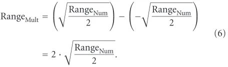
Assume we have signed numbers and a numerical range (RangeNum) symmetric to zero. To avoid a range overflow duringmultiplicationof two numbers, each variable is scaled to the smaller range RangeMultdefined as
RangeMult=
RangeNum 2
−
−
RangeNum 2
=2·
RangeNum
2 .
(6)
Additionally, the so-called Headroom (in percent) for each variable can be defined. Together with the physical ranges PhyRange, the number range RangeMult (6), and the Head-room, the scaling factorsi for each element ofxd,y, andu variables can be computed:
si=
PhyRangei
RangeMult·1−(0,01·Headroom). (7)
LetS = diag(si) be the diagonal matrices composed of the scaling factorssi. With these scaling matrices, the new dis-crete and scaled system matrices are as follows:
As,d=S−xd1·Ad·Sxd,
Bs,d=S−xd1·Bd·Su,
Cs,d=S−y1·Cd·Sxd,
Ds,d=S−y1·Dd·Su.
(8)
The scaling of the matrices withSis necessary since input, output, and state vectors are also scaled with S. Neverthe-less, the coefficients of the matricesAs,d,Bs,d,Cs,d, andDs,d could be out of the selected number range because only the ranges of the inputs, outputs, and states were taken into consideration until now. To avoid overflow, each equation has to be prepared to allow the representation of the co-efficients within RangeMult. For this, one uses bit shifting operations to allow an efficient implementation of multi-plications. Right shifting causes reduced precision with the controller evaluation. So the choice of the word length em-ployed with arithmetic operations is closely related to the shift amount (ShiftAB,ShiftCD):
As,d=2ShiftAB·As,d,
Bs,d =2ShiftAB·Bs,d,
Cs,d=2ShiftCD·Cs,d,
Ds,d=2ShiftCD·Ds,d.
(9)
The right shift operation leads to the new matricesAs,d,
Bs,d,Cs,d, andDs,d. Since the matrices contain only fixed val-ues, shifting must be doneonly onceand guarantees that no overflows will occur during computations. To obtain correct values, the computation results must be corrected by a final left shift operation (note that ShiftAB and ShiftCD are nega-tive)
x(k+ 1)=2−ShiftAB·A
s,d·x(k) +Bs,d·u(k)
, (10)
y(k)=2−ShiftCD·C
s,d·x(k) +Ds,d·u(k)
, (11)
x(k)=x(k+ 1). (12)
The choice of the word length is a compromise between the numerical precision of the controller and the hardware re-sources required for the implementation. It is useful to pro-vide different word lengths for states, inputs, outputs, and internal multiplication/addition registers. Before hardware synthesis, our approach provides a simulation-based selec-tion of the number of bits for the controller variables before starting the target-specific synthesis of the controller. For the modeling and simulation of scaled state-space controllers, we designed a component for our existing simulation environ-ment CAMeL (Computer-Aided Mechatronics Laboratory) [7], with a word length that is tunable during runtime.
3. AUTOMATED DESIGN FLOW
Modelling of the control path
Analysis, simulation
Controller synthesis
Discretization
Scaling
Programming microcontrollerOR
Synthesis of hardware
Prototyping
C
o
nt
ro
l
eng
ineer
ing
T
ransfor
mat
ion
R
ealization
Describing the behaviour of the control path by using ordinary differential equations
Analysis of eigenvalues, frequency response etc.; validation of plausibility; and adjusting the model to the real world Design of the controller as linear
time-invariant continuous state system; and simulation of the complete control loop Transforming the differential equations of the controller state system to difference equations
Scaling the system values (input, output, state) from physical range to numerical range ([−1,+1[)
Implementing controller as algorithm and compilation for microcontroller or synthesis of hardware controller Realization of target platform (e.g., microcontroller or FPGA); hardware in the loop simulation test
Figure3: Design flow.
determining the scaling factors, the design flow down to the hardware is fully automatic.
4. IMPLEMENTATION OF LINEAR CONTROL SYSTEMS ON RECONFIGURABLE HARDWARE
We compare two different implementations of digital control systems: a hardware controller and a software program run-ning on a microprocessor. To prototype the system, an Aptix System Explorer (http://www.aptix.com/products/mp3.htm) with a Xilinx Virtex FPGA module (XCV2000E, [8]) is used. The FPGA is connected to the control path via a D/A con-verter and signal transducers and can be configured either for the hardware or for the software solution.
4.1. Hardware implementation
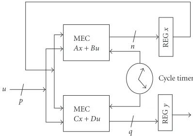
The task of the controller hardware is to compute (10), (11), and (12). Here, x(k), x(k+ 1), u(k), and y(k) are vectors and As,d,Bs,d,Cs,d, andDs,d are the matrices obtained af-ter discretization and scaling. All matrix and vector elements are fixed-point values. Since both (10) and (12) have exactly the same structure, they can be computed in parallel on two identical units called MECs (matrix equation calculators). Each equation is computed once per sample period which is an integral multiple of the clock period.
The top-level structure of our linear controller design is shown inFigure 4. Besides the MECs, we have two vector reg-isters, one for the controller state (REGx) and one for the output (REGy). Thecycle timeris a local state machine for synchronizing the MECs.
u p
MEC
Ax+Bu
MEC
Cx+Du
n
q
Cycle timer
REG
x
REG
y
Figure4: Architecture of the controller hardware.
The MEC components are identical and compute equa-tions of the general form
c=M a+N b (13)
withN andMmatrices and a,b, andcvectors. Internally, an MEC (Figure 5) consists of a vector adder and two scalar multipliers, each of which computes a matrix-vector product as a sequence of scalar multiplications of the form
c=ab=
a1 .. . an
·
b1 .. . bn
a
b
Vector gen
M, N
LineM
LineN
Controller
Scalar mul
Scalar mul
Vector add c
Figure5: Architecture of the MEC unit.
Each scalar multiplier in turn consists of a number of booth-style integer multipliers. The matricesMandNare constant and hard coded in thevector genunit which provides the ma-trices line by line to the scalar multipliers. The design is com-pletely specified in VHDL and parameterizable with respect to the parametersp,n,q, and the word length, wherepis the dimension of the input vectoru,nthe number of controller states, andqthe dimension of the output vector y. The re-source usage of our sample implementation is discussed in Section 5.2.
4.2. Software implementation
The software implementation is based on the S-core micro-processor [9] (Figure 6). The S-core micro-processor design is code-compatible with the Motorola M-core M200 design [10]. It is a 32-bit single-address RISC machine with load/store archi-tecture and a performance of up to 50 MIPS. The processor is available as VHDL core and can be implemented in different silicon technologies. For the case study in this paper, it is syn-thesized for the Xilinx Virtex FPGA family and an Infineon CMOS gate array technology. Programming of the S-core is supported by the GNU C/C++ tools of the M-core.
5. INVERSE PENDULUM: AN APPLICATION STUDY
5.1. Experiment
Using the design flow presented in Section 3 and the hardware structure proposed in Section 4, we have imple-mented an FPGA-based linear controller for an inverse pen-dulum.
The mechanical construction of the pendulum is shown in Figure 7 and the physical model is given inFigure 8. A crab is mounted on a spindle which is rotated by a precision motor. The speed of the motor is simply voltage-controlled. The pendulum mounted on the crab can swing around by 360 degrees. The spindle as well as the axis where the pen-dulum is mounted on are connected to incremental trans-mitters which generate pulses if the spindle rotates or the pendulum moves. These pulses are used for determining the crab position (related to a zero position) and the angle of the pendulum. The task of the linear controller is to
bal-S-core
I/O
IRQ
Bus-controller
PC
Address Register
Decoder ALU
Exception decoder
Figure6: Architecture of the S-core RISC processor [9].
Spindle
Crab DC-motor
Tacho generator Pendulum
Incremental-transmitters
Figure7: Case study: mechanical construction of the pendulum.
z x mG
xG
FK m K
xK
ϕG
IG
Figure8: Case study: mechanical model.
ance the pendulum up-side-down over the crab, even if the pendulum balance is interfered with mechanical pulses. The physical model (Figure 8) is used to find the parameters for the mathematical model. The parameterddescribes the frac-tion of the mechanical components,mGandKdescribe the masses of the parts of the mechanical construction, andFKis the force which is given by the DC motor to the spindle.
xGnom
Figure9: Controller structure.
¨
Transforming these equations to the general form
˙
x=Ax+Bu (16)
leads to the matrices
A=
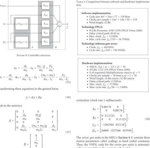
Figure 9illustrates the structure of the controller spec-ified inSection 2. Compared withFigure 2inSection 2, the component A ofFigure 9represents a primitive observer. The differentiators (in A) are necessary to regenerate the state vector. Component B corresponds with the controller-Rin Figure 2and realizes the state controller. For the implemen-tation, this representation must be transformed into the state space representation (matricesA,B,C, andD).
Using the representation from (3) for controller de-sign, we obtain the following controller parameters after
dis-Table1: Comparison between software and hardware implementa-tion.
Software implementation
• Code size: 8n2+ 10n+ 77=129 Byte • Clocks per sample=24n2+ 14n+ 95=219 • Word length: 32 Bit
Technology FPGA:
• #CLBs Processor: 4345 (35% FPGA Virtex 2000)
• Delay critical path: 80.05 ns
• Max. clock:fsys=12 MHz
• Max. cycle rate:fsys/219=54.79 kHz
Technology infineon gate array: • Clock:fsys=160 MHz
• Cycle rate:fsys/219=730.59 kHz
Hardware implementation
• #MUL: 2(p+n)=2(3 + 2)=10
• #CLBs: 1123 (5% FPGA Virtex 2000)
• # of sequential Multiplications: max(n, q)=3
• Clocks per sample=18 max(n, q) + 2=56
• Word length: 16 Bit extern/32 Bit intern
• Delay critical path: 12.838 ns
• Max. clock:fsys=77 MHz • Max. cycle rate: fsys/56=1,3 MHz
cretization (clock rate 1 millisecond):
Ad=
26860 1327446 447044.
(18)
Thevector genunits in the MECs (Section 4.1) contain these matrix parameters (after scaling) as hard coded constants. Thus, the VHDL code for thevector genunits is automati-cally generated from the control path model.
5.2. Results
The experiment shows clearly the advantages of an im-plementation of digital linear controllers in reconfigurable hardware for the same flexibility as a software implemen-tation; it is possible to implement larger control systems as in software with the same throughput. By exploiting more parallelism in the MEC units (Section 4.1) (e.g., by using more multipliers), it is possible to increase further the sam-ple rate of the hardware architecture. The implicit parallelism of the reconfigurable hardware allows real-time computation with high sampling rates. This property leads to controllers which are more stable than software controllers. Addition-ally, it is possible to implement also nonstandard fixed-point number ranges in difference to standard floating-point num-bers of software implementations for higher precision.
6. CONCLUSIONS
The paper shows how reconfigurable hardware can be used for the implementation of digital linear controllers that re-quire a high amount of digital signal processing. We have presented a new design flow for automatic synthesis of dig-ital linear controllers from the mathematical description of the control path. Furthermore, the differences between hard-ware and softhard-ware solutions and their computational com-plexity were discussed for an example of an inverse pen-dulum controller. The paper shows that it is possible to implement application-specific hardware structures with a flexibility comparable to the flexibility of software solu-tions.
Future work will show that this concept can be used for the implementation of self-adapting systems. We plan to ap-ply the described approach to a real-life example of a mecha-tronic train control system. This case study will be more complex than in this paper since the following additional technical requirements have to be considered:
(a) How can reconfigurable hardware be used for imple-mentation of safety-critical systems?
(b) Can FPGA implementations perform dynamic switch-ing between different controllers?
In this context, dynamic reconfiguration of FPGA might be of high importance.
ACKNOWLEDGMENT
We would like to thank Aptix Corporation (San Jose, Calif, USA) for the technical support during the prototype imple-mentation of our methodology using the Aptix system Ex-plorer MP3C.
REFERENCES
[1] T. B. Goh, Z. Li, B. M. Chen, T. H. Lee, and T. Huang, “Design and implementation of a hard disk drive servo system using robust and perfect tracking approach,” IEEE Transactions on Control-Systems Technology, vol. 9, no. 2, pp. 221–233, 2002.
[2] S. Koganezawa and T. Hara, “Development of shear-mode piezoelectric microactuator for precise head positioning,” Fu-jitsu Scientific & Technical Journal, vol. 37, no. 2, pp. 212–219, 2001.
[3] H. Toshiyoshi, “Microactuators for hard disk drive head po-sitioning,” in The 30th Seiken Symposium on Micro/Nano Mechatronics, Komaba, Meguro-ku, Tokyo, Japan, March 2002.
[4] R. Cumplido-Parra, S. R. Jones, R. M. Goodall, F. Mitchell, and S. Bateman, “High performance control system proces-sor,” inProc. 3rd Workshop on System Design Automation (SDA ’00), pp. 60–67, Dresden, Germany, March 2000.
[5] K. Danne, “Implementierung digitaler Regelungen in Hard-ware,” Project Thesis (FB14/DATE) (in German), University of Paderborn, Paderborn, Germany, October 2000.
[6] O. F¨ollinger,Regelungstechnik, H¨uthig, Heidelberg, Germany, 1994.
[7] M. Hahn and T. Koch, “CAMeL-View—Ein Werkzeug zum integrierten CAD-gest¨utzten Entwurf mechatronischer Sys-teme,” inSimulation im Maschinenbau, SIM ’2000, Dresden, Germany, 2000.
[8] Xilinx, Virtex Series Configuration Architecture User Guide, September 2000.
[9] H. Kalte, D. Langen, E. Vonnahme, A. Brinkmann, and U. R¨uckert, “Dynamically reconfigurable system-on-programmable-chip,” inProc. 10th Euromicro Workshop on Parallel, Distributed and Network-Based Processing (PDP ’02), pp. 235–242, Gran Canaria Island, Spain, January 2002. [10] Motorola. M-Core Reference Manual.
Marcus Bednarareceived his Diploma de-gree in computer science in 1998 from the University of Kaiserslautern, Germany. From 1999 to 2002, he was a Researcher and Ph.D. student with the group of Pro-fessor J. Teich (Computer Engineering Lab-oratory) at the University of Paderborn, Germany. Since 2003 he is with the Com-puter Science Institute of the Friedrich-Alexander University Erlangen-Nuremberg
(Hardware-Software-Co-Design group). His research interests are in the area of design automation of VLSI processor ar-rays, their efficient mapping to reconfigurable architectures, dy-namic reconfiguration, and FPGA-based systems for elliptic curve cryptography.
Klaus Danne received his Diploma de-gree in engineering computing in 2002 from the University of Paderborn, Ger-many. As a Ph.D. student and member of the Graduiertenkolleg “Automatic Configu-ration in Open Systems” of the Heinz Nix-dorf Institute of Paderborn University, he was a Researcher in the group of Professor J. Teich (Computer Engineering Laboratory) in 2002. Since 2003 he is with the group of
Markus Deppe studied mechanical engi-neering at the University of Paderborn, Ger-many. He received his Diploma degree in engineering in 1997. Since then he has been a Research Assistant at the Mechatron-ics Laboratory Paderborn (MLaP). His re-search area is the multiobjective parame-ter optimization combined with distributed real-time simulation of mechatronic sys-tems.
Oliver Oberschelpworked as a trained ma-chine fitter before receiving the university diploma in engineering. After that he stud-ied mechanical engineering at the Univer-sity of Paderborn, Germany. He received his diploma in 1998. Since then he has been a Research Assistant at the Mecha-tronics Laboratory Paderborn (MLaP). His research area is design and simulation of mechatronic systems in the context of self-optimizing systems.
Frank Slomkastudied electrical engineer-ing and microelectronics at the Technical University of Braunschweig, Germany. Af-ter receiving the diploma degree in 1993, he was with the Bosch Telecom. At Bosch, he worked as a software Engineer for digital cordless telephone systems (DECT). From 1996 to 2001, he was with the Rapid Proto-typing and Hardware/Software-Co-Design group (Computer Networks and
Commu-nication Systems chair), University of Erlangen-Nuremberg. From 2001 to 2002, he was a member of the research staffat the group DATE at the University of Paderborn. Since 2003, he is an Assistant Professor for embedded system design at the University of Olden-burg.
J¨urgen Teich received his M.S. degree in 1989 from the University of Kaiserslautern (with honours). From 1989 to 1993, he was a Ph.D. student at the University of Saar-land, Saarbr¨ucken, Germany from where he received his Ph.D. degree. In 1994, Dr. Te-ich joined the DSP design group of Prof. E. A. Lee and D. G. Messerschmitt in the Department of Electrical Engineering and Computer Sciences (EECS) at UC Berkeley