The Thirty-Third AAAI Conference on Artificial Intelligence (AAAI-19)
Distribution-Based Semi-Supervised Learning for Activity Recognition
Hangwei Qian,
†‡§Sinno Jialin Pan,
†Chunyan Miao
†‡£ †School of Computer Science and Engineering‡Joint NTU-UBC Research Centre of Excellence in Active Living for the Elderly §Interdisciplinary Graduate School
£Alibaba-NTU Singapore Joint Research Institute
Nanyang Technological University, Singapore [email protected],{sinnopan, ascymiao}@ntu.edu.sg
Abstract
Supervised learning methods have been widely applied to ac-tivity recognition. The prevalent success of existing methods, however, has two crucial prerequisites: proper feature extrac-tion and sufficient labeled training data. The former is im-portant to differentiate activities, while the latter is crucial to build a precise learning model. These two prerequisites have become bottlenecks to make existing methods more practi-cal. Most existing feature extraction methods highly depend on domain knowledge, while labeled data requires intensive human annotation effort. Therefore, in this paper, we propose a novel method, named Distribution-based Semi-Supervised Learning, to tackle the aforementioned limitations. The pro-posed method is capable of automatically extracting powerful features with no domain knowledge required, meanwhile, al-leviating the heavy annotation effort through semi-supervised learning. Specifically, we treat data stream of sensor readings received in a period as a distribution, and map all training dis-tributions, including labeled and unlabeled, into a reproduc-ing kernel Hilbert space (RKHS) usreproduc-ing the kernel mean em-bedding technique. The RKHS is further altered by exploit-ing the underlyexploit-ing geometry structure of the unlabeled distri-butions. Finally, in the altered RKHS, a classifier is trained with the labeled distributions. We conduct extensive experi-ments on three public datasets to verify the effectiveness of our method compared with state-of-the-art baselines.
Introduction
Human activity recognition has spurred a great deal of in-terest with a wide spectrum of real-world applications, such as security, personalized health monitoring and assisted liv-ing (Janidarmian et al. 2017; Bullliv-ing, Blanke, and Schiele 2014; Lara and Labrador 2013; Frank, Mannor, and Precup 2010; Avci et al. 2010). Generally, there are two types of sce-narios: wireless-sensor-based and video-based. In this work, we focus on wireless-sensor-based activity recognition sce-narios. In these scenarios, the data is often in the form of a continuous multivariate time series from multiple sensors. Therefore, the data needs to be divided into segments first, each of which corresponding to a single label. Traditionally, it requires intensive annotation effort with the starting and ending times of each activity. Further, in order to increase the expressiveness of data, feature extraction is commonly
Copyright c2019, Association for the Advancement of Artificial Intelligence (www.aaai.org). All rights reserved.
applied to each segment. Extracted features are then fed into a classifier to recognize different activities. Note that feature extraction and large amount of labeled training data are cru-cial in the process, which are discussed in detail hereinafter. It is well-known that good features can help to discrimi-nate different classes of activities, by increasing the expres-siveness of each activity. Generally, feature extraction ap-proaches can be classified into two categories: statistical and structural (Lara and Labrador 2013). Structural features take into account the overall information of the data. For exam-ple, SAX method transforms continuous data into discrete symbolic strings (Lin et al. 2007); ECDF method preserves the overall shape and spatial information of time series data (Hammerla et al. 2013; Pl¨otz, Hammerla, and Olivier 2011). Therefore, domain knowledge is highly required for structural features. Statistical features, on the other hand, aim to capture statistical information underlying each time-series segment. There are also around twenty commonly used handcrafted statistical features which are proven to be beneficial practically, including orders of moments (mean, variance, skewness, etc), median, etc (Janidarmian et al. 2017). Major limitations of statistical features are the flexi-bility of handcrafted features and the involvement of domain knowledge. Recently, Qian, Pan, and Miao (2018) proposed the SMMAR approach, which is capable of automatically extracting all orders of moments as statistical features for activity recognition.
methods adopt handcrafted features.
In this paper, we propose a novel semi-supervised learn-ing method, namely Distribution-based Semi-Supervised Learning (DSSL), to free the intensive effort on feature engi-neering by using the kernel mean embedding technique for distributions (Berlinet and Thomas-Agnan 2011). To elab-orate, we treat data stream of sensor readings received in a period as a probability distribution. Modeling input in-stances as probability distribution is a new and promising machine learning paradigm, and some methods have been successfully developed in the supervised learning manner, e.g., Support Measure Machines (SMMs) (Muandet et al. 2012; 2017). Recently, Qian, Pan, and Miao (2018) pro-posed a framework based on SMMs for activity recogni-tion, which is known as SMMAR. A major advantage of SMMARover other supervised learning methods for activ-ity recognition is the capabilactiv-ity of automatically extracting all the orders of statistical moments as features to repre-sent each input instance. Our proposed method, DSSL, is an extension of SMMAR in the semi-supervised learning manner. Compared with SMMAR and other supervised or semi-supervised learning methods for activity recognition, our contributions are 4-fold:
• Compared with other supervised or semi-supervised learning methods, DSSL is able to represent each in-stance, i.e., data stream of a period, using all the orders of statistical moments implicitly and automatically, which contains rich information to distinguish activities.
• Compared with SMMAR, DSSL relaxes its full supervi-sion assumption, and is able to exploit unlabeled instances to learn an underlying data structure. With the learned structure and a few labeled instances, DSSL is able to learn a precise classifier for activity recognition.
• Most existing works on learning with distributions are supervised. To the best of our knowledge, DSSL is the first attempt on semi-supervised learning with distribu-tions. Moreover, we provide theoretical analysis proving that DSSL is valid for semi-supervised learning in a re-producing kernel Hilbert space (RKHS).
• Extensive experiments are conducted to demonstrate the superior performance of DSSL over a number of state-of-the-art baselines.
Other Related Work
Limited labeled training data is insufficient to train a good classifier due to the cold start problem of supervised learn-ing. Semi-supervised learning approaches are appealing in practice since they require only a small fraction of labeled training data with a large amount of easily obtained unla-beled data (Chapelle, Schlkopf, and Zien 2010; Zhu 2005). Among existing semi-supervised learning approaches, man-ifold regularization (Sindhwani, Niyogi, and Belkin 2005) and wrapping kernels using point cloud (Belkin, Niyogi, and Sindhwani 2006) are two classic methods, which incorpo-rates the manifold structure underlying both unlabeled and labeled data into the learning of Support Vector Machines (SVMs).
In the context of activity recognition, Stikic, Larlus, and Schiele (2009) proposed a multi-graph based semi-supervised approach named GLSVM, where each graph propagates different information of activities. Different graphs are then combined to improve label propagation in graphs. After that, an SVM classifier is trained by using both the initially labeled training data and the propagated la-bels. Matsushige, Kakusho, and Okadome (2015) proposed a semi-supervised kernel logistic regression method for ac-tivity recognition, denoted by SSKLR, which extends ker-nel logistic regression into semi-supervised fashion, and solves the problem by the Expectation-Maximization al-gorithm. Yao et al. (2016) proposed a robust graph-based semi-supervised method named RSAR to tackle the intra-class variability in activities across different subjects. The RSAR method extracts the intrinsic shared subspace struc-tures from activities with the assumption that intrinsic re-lationships have invariant properties thus are less sensi-tive with varying subjects. In (Naz´abal et al. 2016), a new Bayesian model is proposed to tackle the scenario with a very low number of sensors. The dynamic nature of human activities are further modeled as a first-order homogeneous Markov chain. Our proposed DSSL is a unified framework that naturally inherits the spirit of learning from distributions and manifold learning.
Preliminaries
Support Measure Machines In supervised learning with distributions, we are given a set of labeled data{Xi, yi}ni=1,
whereXi={xij}nj=1i andn
0
ismay vary across differentxi. The goal is to learn a classifierfto map{Xi}’s to{yi}’s. In SMMs (Muandet et al. 2012), eachXiis mapped to a func-tional in a RKHS Hvia kernel mean embedding (Berlinet and Thomas-Agnan 2011) as µPi = Exij∼Pi[k(xij,·)],
where k(·,·)is a characteristic kernel associated with the RKHSH. It has been proven that if the kernel is character-istic, then an arbitrary probability distributionPiis uniquely represented by an elementµP
iin the RKHS, which
implic-itly captures all orders of statistical moments ofXi. The inner product, i.e., a linear kernel, of two distribu-tions, which measures their similarity, can be defined as
hµP
i,µPji =
1
ninj
Pni
a=1 Pnj
b=1k(xia,xjb). One can also define a nonlinear kernel of µPi andµPj to capture their nonlinear relationships via
˜
k(µPi,µPj)H˜ =hψ(µPi), ψ(µPj)i, (1)
where˜k(·,·)is the nonlinear kernel induced by the nonlinear feature mapψ(·), andH˜is the corresponding RKHS.
To train a classifier from{Xi}’s to{yi}’s, SMMs define the optimization problem by learningf ∈H˜that minimizes the following regularized risk functional
1
n
n
X
i=1
`(µPi, yi, f) + Ω(kfkH˜), (2)
Random Fourier Features Approximation The kernel embedding technique of distributions used in SMMs is com-putationally expensive as it requires to compute kernel ma-trices. This makes it impractical in some real-world appli-cations when the size of the dataset is large. To scale up SMMs, Qian, Pan, and Miao (2018) proposed an accelerated version using Random Fourier Features to construct an ex-plicit feature map instead of using the kernel trick. Based on Bochner’s Theorem (Rahimi and Recht 2007), a continuous, shift-invariant positive definite kernel k(x,x0)can be lin-earized by using the randomized feature mapz:Rd →RD
as
k(x,x0) =hφ(x), φ(x0)i ≈z(x)>z(x0), (3)
where the inner product of explicit feature maps can uni-formly approximate the kernel values without the kernel trick, and the random Fourier features are generated by:
zw(x) = √
2cos(w>x+b), (4)
wherew ∼ p(w), which isk(·,·)’s Fourier transform dis-tribution onRD, andbis sampled uniformly from[0,2π]. It
can be proven thatk(x,x0) = E(zw(x)>zw(x0))for all x andx0. In practice,Dcan be small, which enables SMMs to handle large-scale datasets.
The Proposed Methodology
Problem Statement
In our project setting of activity recognition, we are given a set of l labeled segments data {Xi, yi}li=1, and a set of u =n−l unlabeled segments{Xi}ii==nl+1as training data
obtained by applying segmentation methods on the raw data, whereXi = [xi1...xini]∈R
d×ni,y
i ∈ {1, ..., L},lu, andni may vary across different segments. The goal is to make use of both labeled and unlabeled segments to learn a classifier from each segmentXto its corresponding labely. Following (Qian, Pan, and Miao 2018), each segmentXi, including both labeled and unlabeled, is treated as asample of ni data points drawn from an unknown distributionPi. Kernel mean embedding is then applied to map eachXi to an elementµPiin a RHKS. In practice, to make the learning process more efficient, random Fourier features are used to approximate the nonlinear feature map induced by the kernel of the RKHS viaµPi =n1
i
Pni
j=1z(xij).whereµPi ∈R
D.
Therefore, our goal becomes to learn a classifierf : µP →
yifrom{µPi, yi}li=1and{µPi}
i=n i=l+1.
Distribution-based Semi-Supervised Learning
Borrowing the idea from manifold regularization (Belkin, Niyogi, and Sindhwani 2006) and the technique on warp-ing data-dependent kernels (Sindhwani, Niyogi, and Belkin 2005), we aim to incorporate the underlying manifold struc-ture of both labeled and unlabeled data into the learning of a classifier via warping a RKHS. Specifically, we wrap the RKHS H˜ defined in (1) to another RKHS H˘ by leverag-ing unlabeled trainleverag-ing segments or distributions to reflect the underlying geometry of {ψ(µP
i)}’s. Notations on
dif-ferent kernels and their corresponding RKHSs used in this
Table 1: Notations of different kernels used in the paper
Kernel Space Descriptions
k H kernel mean embedding of distributions
˜
k H˜ kernel on the embedded distributions
˘
k H˘ data-dependent kernel constructed based
on˜kfor semi-supervised learning
paper are summarized in Table 1. The new RKHSH˘ is as-sociated with the new kernelk˘, which is data-dependent for semi-supervised learning. We will discuss how to achieve the kernel as well as the resulting new space later. Here, we assume the new kernel˘kis constructed, then the revised op-timization problem overH˘is formulated as
f∗= arg min
f∈H˘
1
l
l
X
i=1 `(µP
i, yi, f) +kfk
2 ˘
H, (5)
where`(·)is the loss function. Note the objective function looks similar to that in the supervised learning setting in (2). However, in (5) the RKHS, where the functional to be op-timized isH˘, which is influenced by both labeled and un-labeled distributions, while the RKHS in (2) is H˜, which is defined by labeled distributions only. The new optimiza-tion probelm raises a potential problem:fis to be learned in
˘
H, while the input space ofµPi isH. As these RKHSs are not the same, how to calculate the loss function remains a problem. To sum up, in order to solve the optimization prob-lem (5), three crucial questions need to be answered:
• How to construct the data-dependent kernelk˘by incorpo-rating unlabeled training data?
• Is the new spaceH˘valid?
• How to calculate the loss function given µP ∈ Hand
f ∈H˘are not in the same space?
In the following, we investigate the questions one by one.
1) Construction of the Data-dependent Kernel˘k Since unlabeled data may shed light on the underlying structure and manifolds of all data, now the problem becomes how to appropriately construct such a valid RKHSH˘ fromH˜to achieve so. We first defineH˘to be the space of functionals fromH˜ with the following modified inner product:
hf, giH˘ ∆
=hf, giH˜+hSf, SgiV, (6)
whereV is a linear space andS: ˜H → Vis a bounded lin-ear operator. The first term in (6) is the common definition of inner product between two functionals, while the second term with the operator S reflects that unlabeled embedded distributions alter our beliefs in the overall structure. De-note byf(µ) = (f(µP1), ..., f(µPn)), we havehSf, SfiV=
f(µ)Mf(µ)>withM being a positive semidefinite matrix.
2) Validity ofH˘
Theorem 1. H˘is a valid RKHS.
3) Loss Function Calculation Based on Theorem 1, we have the following propositions.
Proposition 1. H˘ = ˜H.
The two spaces are the same if each of the space is the subset of the other space. Although the two spaces are the same, the kernels therein are not identical. However, they are connected due to the involvement of unlabeled distributions.
Proposition 2. K˘ = (I+ ˜KM)−1K,˜ whereK˜ withK˜ij = ˜
k(µPi,µPj)is the kernel matrix forH˜ onµPi’s, andK˘ is the kernel matrix in the altered spaceH˘.
Note that detailed proofs and derivations of theorems and propositions introduced in this section can be found in the next section. The complexity of the above kernel seems to be a potential problem when the data scales up, since it involves matrix multiplication as well as matrix inversion. However, when conducting experiments on large scale activity recog-nition datasets, the problem actually is not severe in practice. The reason is that the entries of kernels are dependent on the number of distributions, i.e., number of segments, each con-taining a repetition of activity, instead of the number of total instances, i.e., one entry for each timestamp equivalent to the product of # sample and # instances per sample. Other feasible solutions to further alleviate this problem include matrix factorization, low-rank approximation (Bach and Jor-dan 2005), etc. Data selection or feature selection (Nie et al. 2010) can be conducted on training data beforehand to keep a small fraction of key training data. The proposed method can be further developed in an online learning fashion (Hoi, Wang, and Zhao 2014), so that the matrix are maintained in a small scale.
Note that the choice of M is crucial regarding how to properly incorporate unlabeled embedded distributions. In this paper, we setM to beM = rL2,whereris a scalar andL=D−W is the Laplacian matrix, which is widely used in semi-supervised learning (Sindhwani, Niyogi, and Belkin 2005; Belkin, Niyogi, and Sindhwani 2006) to model the geometry structure underlying the data. To be specific,
Wij =exp
−kµPi−µPjk 2
2σ2
ifµPiandµPj are connected in
the graph, andDis the diagonal matrix withDii=PjWij. Based on the following Theorem 2 (whose derivations are at the end of the paper), the solution for the optimization prob-lem in (5) can be expressed as a linear combination of the functionals{˘k(µPi),·}l
i=1as
f∗(µP) =
l
X
i=1
αik˘(µP,µPi). (7)
Theorem 2 (Representer Theorem for the pro-posed DSSL method). Given l labeled distributions
{(P1, y1), ...,(Pl, yl)} ∈ P × R, a loss function ` : (P ×R2)l → R∪ {+∞} and a strictly
monoton-ically increasing real-valued function Ω on [0,+∞), the minimizer of the regularized risk functional
`(P1, y1,EP1[f], ...,Pl, yl,EPl[f]) + Ω(kfkH˘), (8)
admits an expansionf =Pl
i=1αi˘k(µPi,·),whereαi ∈R,
fori= 1, ..., l.
Detailed Proofs
Proof of Theorem 1 Let’s start withH˜ with the kernel˜k. Since H˜ is a complete Hilbert space, and evaluation func-tionals therein are bounded, i.e.,∀µ∈ H, f∈H˜,∃Cµ∈R,
s.t.|f(µ)| ≤CµkfkH˜. Moreover, the bounded operatorSis
bounded by a constantD, i.e.,kSk= sup
f∈H˜
kSfkV
kfkH˜ ≤D. The
completeH˜means every Cauchy sequence in the space con-verges to an element inH˜. Let(fn)be a Cauchy sequence inH˜converging tof, then∀ >0,∃an integerN(), s.t.
m > N(), n > N()⇒ kfm−fnkH˜ <
√
1 +D2.
Now let’s turn toH˘. We need to prove the completeness of the space first. According to the definition in Eq. (6), we obtain that for any Cauchy sequence inH˘,
kfm−fnkH2˘ =kfm−fnk2H˜+kS(fm−fn)k2V
≤ kfm−fnk2H˜+D2kfm−fnk2H˜
=⇒ kfm−fnkH˘ ≤ p
1 +D2kf
m−fnkH˜
<p1 +D2×√
1 +D2 =.
Hence H˘ is complete since every Cauchy sequence in H˘
converges to an element in H˘. Moreover, H˘ is bounded based on the property that any Cauchy sequence is bounded (Berlinet and Thomas-Agnan 2011, Lemma 5). This completes the proof.
Proof of Proposition 1 Firstly, we decomposeH˘ to two orthogonal parts as
˘
H=span{k˘(µP1,·), ...,k˘(µPl,·)} ⊕H˘⊥,
whereH˘⊥ vanishes at all labeled embedded distributions, i.e.,
∀f ∈H˘⊥, i∈ {1, ..., l}, f(µ
Pi) = 0. (9)
Accordingly Sf = 0, which means hf, giH˘ =
hf, giH˜,∀f ∈H˘⊥, g∈H˘. Moreover,
f(µP) =hf,˘k(µP,·)iH˘ =hf,k˜(µP,·)iH˜
=hf,k˜(µP,·)iH˜+hSf, Sk˜(µP,·)iV
=hf,k˜(µP,·)iH˘.
Thus, we have
∀f ∈H˘⊥, hf, k˜(µ
P,·)−˘k(µP,·)iH˘= 0. (10)
That isk˜(µP,·)−˘k(µP,·) ∈ ( ˘H⊥)⊥. By substituting (9) into (10), we obtain˜k(µPi,·)∈( ˘H⊥)⊥, ∀i, which means
span{˜k(µPi,·)}l
i=1⊆span{k˘(µPi,·)}
l
i=1. (11)
Secondly, we decompose H˜ as H˜ =
span{k˜(µPi,·)}l
i=1⊕H˜⊥. Similarly, we have
AsSf = 0, we havehf, giH˜ =hf, giH˘, and
f(µP) =hf,˜k(µP,·)iH˜ =hf,k˘(µP,·)iH˘
=hf,k˘(µP,·)iH˜+hSf, S˘k(µP,·)iV
=hf,k˘(µP,·)iH˜.
Therefore, we havehf, ˘k(µP,·)−k˜(µP,·)iH˜ = 0. Since f ∈ H˜⊥, it becomes hf,˘k(µ
P,·)iH˜ = 0, i.e.,k˘(µP,·) ∈
( ˜H⊥)⊥. Therefore, we have
span{˘k(µP
i,·)}
l
i=1⊆span{k˜(µPi,·)}
l
i=1. (12)
Finally, by considering both (11) and (12), we conclude that the two spans are the same. This completes the proof.
Proof of Proposition 2 Based on Proposition 1, we have
˘
k(µP,·) = ˜k(µP,·) +
n
X
j=1
βj(µP)˜k(µPj,·), (13)
where the coefficients βj depend onµP. If we can obtain the exact formulation for βj, then we can derive relations between two spaces by explicit forms. To findβj, we use a system of linear equations generated by evaluating˜k(µPi,·)
atµP:
h˜k(µ
Pi,·),k˘(µP,·)iH˘
=h˜k(µ
Pi,·),˜k(µP,·) + n X
j=1
βj(µP)˜k(µPj,·)iH˘
=h˜k(µ
Pi,·),˜k(µP,·) + n X
j=1
βj(µP)˜k(µPj,·)iH˜+˜k
>
µP
iMg,
where ˜k>µ
Pi
= ˜k(µPi,µP1), ...,˜k(µPi,µPn) and
g consists of components gi = k˜(µP,µPi) +
Pn
j=1βj(µP)˜k(µPj,µPi). Then we have the fol-lowing linear equation for the coefficients β(µP) = (β1(µP), ..., βn(µP))>:
−M˜kµ
P = (I+M
˜
K)β(µP). (14)
Based on (13) and (14), we obtain the following explicit form for˘k(·,·):
˘
k(µP
i,µPj) = ˜k(µPi,µPj)− ˜
k>µ
Pi
(I+MK˜)−1M˜kµP
j.
The above equation can be written in the following concise matrix form:
˘
K= ˜K−K˜(I+MK˜)−1MK.˜ (15)
It can be shown that by applying the Sherman-Morrison-Woodbury (SMW) identity, (15) can be further rewritten as
˘
K= (I−K˜(I+MK˜)−1M) ˜K= (I+ ˜KM)−1K.˜ (16)
This completes the proof.
Proof of Theorem 2 Any functional f ∈ H˘ can be uniquely decomposed into a component fµ in the
space spanned by the kernel mean embedding fµ =
Pl
i=1αik˘(µPi,·), and a componentf⊥orthogonal to it, i.e.,
hf⊥,˘k(µPj,·)i= 0,∀j∈ {1, ..., l}. Therefore, we have
f =fµ+f⊥= l
X
i=1
αik˘(µPi,·) +f⊥.
Thus, for allj, we can further induce that
EPj[f] =
* l
X
i=1
αi˘k(µPi,·) +f⊥, k˘(µPj,·)
+
=
* l
X
i=1
αi˘k(µPi,·),k˘(µPj,·)
+
.
This indicates the loss function term in (8) does not depend onf⊥. Besides, the second termΩ(·)in (8) is strictly mono-tonically increasing, so we have
Ω(kfkH˘) = Ω l X i=1
αi˘k(µPi,·) +f⊥
H˘ ! = Ω v u u t l X i=1
αi˘k(µPi,·)
2 ˘ H
+kf⊥k2H˘ ≥Ω l X i=1
αi˘k(µPi,·)
˘ H ! ,
where the equality holds if and only iff⊥ = 0. Therefore, the first term in (8) is independent of f⊥ and the second term reaches its minimum whenf⊥= 0. Consequently, any minimizer must take the formf =fµ=P
l
i=1αik˘(µPi,·). This completes the proof.
Experiments
We conduct experiments on 3 sensor-based activity datasets. The statistics are listed in Table 2. Skoda records 10 gestures in car maintenance scenarios with 20 acceleration sensors being put on the arms of the subject (Stiefmeier, Roggen, and Tr¨oster 2007). Each gesture is repeated around 70 times. The transitions between two gestures are labeled as Null class, which are also considered as activities. WISDM uses accelerometer sensors embedded in the phones to collect six regular activities: jogging, walking, ascending stairs, de-scending stairs, sitting and standing (Kwapisz, Weiss, and Moore 2010). HCI composes of gestures with the hand describing different shapes: a circle, a square, a pointing-up triangle, an pointing-upside-down triangle, and an infinity sym-bol (F¨orster, Roggen, and Tr¨oster 2009). Each gesture is recorded over 50 repetitions, and about 5 to 8 seconds per repetition. Null class exists as well in HCI dataset.
Experimental Setup
Table 2: Statistics of datasets used in experiments.
Datasets # Sample # Instances per sample # Feature # Class
Skoda 1,447 68 60 10
HCI 264 602 48 5
WISDM 389 705 6 6
score (maF) to evaluate the performance of different meth-ods. All the reported results are the average values together with the standard deviation over 6 random splits for training and testing. Each dataset is randomly split into 3 subsets: la-beled training set, unlala-beled training set and test set. Each subset is set to contain activities of all classes. We set the ratio to be 0.02:0.1:0.88 and fixr= 100. The impact of dif-ferentiatingrwill be discussed later. Different from experi-mental setups in existing papers that set labeled data’s ratio to be quite large (Matsushige, Kakusho, and Okadome 2015; Stikic, Larlus, and Schiele 2009), we deliberately set the la-beled data’s ratio to be extremely small. Hence, our method requires fewer labels and thus more practical with regards to applicability in reality. Evaluations are conducted on the test set. We adopt RBF kernels for all the kernels used in the experiments.
Baselines We compare the proposed DSSL method with the following state-of-the-art methods.
• State-of-the-art supervised methods with various features:
– SVMs (Chang and Lin 2011): as SVM is a vectorial-based classifier, we use mean, variance, etc to generate a feature vector for each segment.
– SAX-a (Lin et al. 2007) treats data as strings, and structural features are extracted. We follow the settings in (Lin et al. 2007) with no dimension reduction. The parameter alphabet size range isa∈ {3,6,9}.
– ECDF-d(Hammerla et al. 2013; Pl¨otz, Hammerla, and Olivier 2011) extractsddescriptors from each sensor’s each dimension.d∈ {5,15,30,45}.
Note that the overall shape and spatial features besides the mean and variance features are concatenated before applying the SVM classifier.
• State-of-the-art supervised method based on distributions, SMMAR(Qian, Pan, and Miao 2018).
• Classic vectorial-based semi-supervised methods:
– LapSVM (Belkin, Niyogi, and Sindhwani 2006) is an extension of SVM with manifold regularization.
– 5TSVM (Chapelle and Zien 2005) is a Transductive SVM by using gradient descent for training. As this is a transductive approach rather than a truly semi-supervised learning approach, we make the test data available in the training phase of this method.
• State-of-the-art semi-supervised methods specifically de-signed for activity recognition:
– SSKLR (Matsushige, Kakusho, and Okadome 2015) is a semi-supervised kernel logistic regression method with Expectation-Maximization algorithm.
– GLSVM (Stikic, Larlus, and Schiele 2009) is a multi-graph method where each multi-graph captures different as-pects of the activities.
Experimental Results
Overall Experimental Results The experimental results are presented in Table 3. The proposed DSSL consistently performs the best on all datasets. DSSL outperforms all the other methods by 5.6%, 17.7%, and 14.4% respectively on three datasets in terms of miF. This favorably indicates the effectiveness of the proposed DSSL. Note that in Table 3, the performances of the comparison methods on WISDM are much worse than those on the other two datasets. This may be due to the data complexity caused by the large number of subjects in WISDM. On datasets Skoda and HCI, the per-formance ranking is DSSL>SMMAR >SVMs≈ECDF
> SAX, which reveals that 1) distribution-based methods are more capable of distinguishing different activities; 2) feature extraction plays an important role and string-based data representation in SAX is not that proper for activity data compared to ECDF; 3) with the increase of descriptor
d, the performance of ECDF is increasing in HCI dataset while decreasing in Skoda and WISDM, meaning ECDF may be task-dependent. However, note that SMMAR per-forms the worst on WISDM dataset, which illustrates that distribution-based methods are more dependent on the num-ber of labeled data than vectorial-based methods. This in-deed reflects the motivation of our proposed method. Never-theless, DSSL does not suffer from this limitation ascribed to its semi-supervised fashion. For semi-supervised methods, the ranking is DSSL>LapSVM≈GLSVM≈ 5TSVM>
SSKLR, which demonstrates the prevalence of graph-based methods over logistic regression method for activity data.
Impact of Ratio of Labeled Data To analyze the impact on the proportion of labeled training data, we conduct ex-periments on WISDM dataset. We fix the ratio of test data and unlabeled training data to be 20% and 20% respectively, and alter the ratio of labeled training data to be{0.02, 0.05, 0.1, 0.3, 0.5, 0.7, 0.9}of the rest 60% data. The results are depicted in Figure 1(a). DSSL performs the best under all the ratios. When more labeled training data becomes avail-able, all methods perform better. Moreover, distributional-based method (SMMAR) has larger performance enhance-ment than vectorial-based methods, which further verifies the superiority of learning from distributions.
Impact of Ratio of Unlabeled data We investigate the in-fluence of unlabeled data by fixing the ratio of labeled train-ing data and test data to be 1% and 20%, respectively, and modifying unlabeled training data to be{0.1, 0.3, 0.5, 0.7, 0.9}of the remaining 79% data. Note that supervised meth-ods (SMMAR, SVMs) and transductive methods (5TSVM) perform the same under this setting, while the performances of semi-supervised methods keep increasing with more un-labeled training data as shown in Figure 1(b).
Impact of parameterr In previous experiments, we fix
Table 3: Experimental results on 3 activity datasets (unit: %).
Methods Skoda HCI WISDM
miF maF miF maF miF maF
Vectorial-based supervised
SVMs 85.7±1.8 42.5±0.9 69.7±9.6 69.6±9.4 41.5±5.2 39.6±6.8 SAX 3 39.6±6.3 18.7±2.9 36.0±3.0 34.7±2.5 34.6±1.4 30.6±1.2 SAX 6 37.2±6.1 18.6±2.8 39.7±7.3 38.4±7.9 34.9±3.0 30.5±5.0 SAX 9 40.3±6.5 19.9±3.2 39.8±8.7 37.0±9.2 33.6±2.9 28.8±5.8 ECDF 5 84.2±2.1 41.6±1.0 67.7±10.1 67.6±9.1 42.1±6.3 40.5±7.7 ECDF 15 79.8±1.5 39.2±0.7 68.4±10.4 68.5±9.6 39.4±3.3 36.2±5.7 ECDF 30 72.6±1.2 35.4±0.3 68.6±11.1 68.7±10.5 37.7±2.5 32.6±4.9 ECDF 45 65.7±2.5 31.5±1.3 68.6±11.4 68.6±10.8 36.4±1.4 31.3±3.6
Vectorial-based semi-supervised
LapSVM 89.7±2.1 44.6±1.2 76.1±4.8 76.3±4.7 40.1±3.8 34.5±3.5
5TSVM 85.9±2.7 84.8±2.8 75.4±11.5 75.5±11.2 41.3±5.6 39.4±6.9 SSKLR 25.4±19.3 12.1±2.5 24.2±17.2 18.1±10.1 24.6±17.0 17.3±9.9 GLSVM 89.7±2.1 44.5±1.2 75.7±5.8 75.7±5.7 40.4±3.8 33.9±4.0 Distribution-based supervised SMMAR 93.2±0.9 93.1±1.0 82.2±13.4 78.9±18.4 20.5±3.3 11.7±3.9 Distribution-based semi-supervised DSSL 98.8±0.5 98.8±0.5 99.9±0.2 99.9±0.2 56.5±5.1 55.6±5.0
0 0.1 0.2 0.3 0.4 0.5 0.6 0.7 0.8 0.9
ratio of labeled data 20
30 40 50 60 70
miF (%, log scale)
SMMAR SVM LapSVM
TSVM DSSL
(a) Varying ratios of labeled data.
0.1 0.2 0.3 0.4 0.5 0.6 0.7 0.8 0.9 ratio of unlabeled data
20 30 40 50 60 70
miF (%, log scale)
SMMAR SVM LapSVM
TSVM DSSL
(b) Varying ratios of unlabeled data.
-6 -4 -2 0 2 4 6
log10r
40 45 50 55 60 65
miF (%, log scale)
DSSL best baseline
(c) Impact ofrto the performance.
Figure 1: Performance of DSSL on WISDM under different settings (in miF).
in Fig. 1(c), the performance of DSSL on test data keeps sta-ble whenr∈[10−6,1]. Whenrbecomes larger, the perfor-mance of DSSL begins to decrease. This observation indi-cates thatrbalances the tradeoff between labeled and unla-beled data. Largerrimplies stronger emphasis on unlabeled data. More importantly, under all differentrvalues, DSSL consistently outperforms all other methods. Fig. 1(c) shows the best baseline, i.e., ECDF 5 in WISDM’s case.
0 5 10 15 20
Random feature dimension D 40
50 60
miF (%, log scale)
R-DSSL DSSL best baseline
0 5 10 15 20
Random feature dimension D 0
2 4 6
run time (s)
R-DSSL DSSL
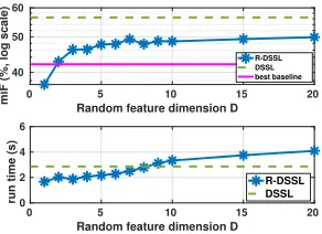
Figure 2: Impact ofDto the performance on WISDM.
Impact on random Fourier feature (RFF) dimension D We analyze how R-DSSL accelerates DSSL with D
-dimensional explicit statistical features. The experiments are conducted on a Linux server with Intel(R) Xeon(R) E5-2695 2.40GHz CPU. As shown in Fig. 2, R-DSSL steadily out-performs the best baseline whenD≥2. Note that R-DSSL performs slightly worse than DSSL due to its approxima-tion nature, however it requires less computaapproxima-tional run time whenD <8compared to DSSL.
Conclusion
In this paper, we propose a semi-supervised learning frame-work, DSSL, for sensor-based activity recognition prob-lems. The proposed DSSL naturally embeds automatic fea-ture extraction and classification in a semi-supervised learn-ing manner. Extensive experiments are conducted on three activity datasets to demonstrate the superiority of DSSL compared with a number of state-of-the-art methods.
Acknowledgments
and the Interdisciplinary Graduate School, Nanyang Tech-nological University under its Graduate Research Schol-arship. Sinno J. Pan thanks the support from the NTU Singapore Nanyang Assistant Professorship (NAP) grant M4081532.020.
References
Avci, A.; Bosch, S.; Marin-Perianu, M.; Marin-Perianu, R.; and Havinga, P. J. M. 2010. Activity recognition using in-ertial sensing for healthcare, wellbeing and sports applica-tions: A survey. InARCS Workshops, 167–176.
Bach, F. R., and Jordan, M. I. 2005. Predictive low-rank decomposition for kernel methods. InICML, 33–40. Belkin, M.; Niyogi, P.; and Sindhwani, V. 2006. Manifold regularization: A geometric framework for learning from la-beled and unlala-beled examples.Journal of Machine Learning Research7:2399–2434.
Berlinet, A., and Thomas-Agnan, C. 2011. Reproducing kernel Hilbert spaces in probability and statistics. Springer Science & Business Media.
Bulling, A.; Blanke, U.; and Schiele, B. 2014. A tutorial on human activity recognition using body-worn inertial sen-sors.ACM Comput. Surv.46(3):33:1–33:33.
Chang, C., and Lin, C. 2011. LIBSVM: A library for support vector machines. ACM Trans. Intell. Syst. Technol 2(3):27:1–27:27.
Chapelle, O., and Zien, A. 2005. Semi-supervised classifi-cation by low density separation. InAISTATS.
Chapelle, O.; Schlkopf, B.; and Zien, A. 2010. Semi-Supervised Learning. The MIT Press.
F¨orster, K.; Roggen, D.; and Tr¨oster, G. 2009. Unsuper-vised classifier self-calibration through repeated context oc-curences: Is there robustness against sensor displacement to gain? InISWC, 77–84.
Frank, J.; Mannor, S.; and Precup, D. 2010. Activity and gait recognition with time-delay embeddings. InAAAI. Guan, D.; Yuan, W.; Lee, Y.; Gavrilov, A.; and Lee, S. 2007. Activity recognition based on semi-supervised learning. In RTCSA, 469–475.
Hammerla, N. Y.; Kirkham, R.; Andras, P.; and Ploetz, T. 2013. On preserving statistical characteristics of accelerom-etry data using their empirical cumulative distribution. In ISWC, 65–68.
Hoi, S. C. H.; Wang, J.; and Zhao, P. 2014. LIBOL: a li-brary for online learning algorithms. J. Mach. Learn. Res. 15(1):495–499.
Janidarmian, M.; Fekr, A. R.; Radecka, K.; and Zilic, Z. 2017. A comprehensive analysis on wearable acceleration sensors in human activity recognition.Sensors17(3):529. Kwapisz, J. R.; Weiss, G. M.; and Moore, S. 2010. Activ-ity recognition using cell phone accelerometers. SIGKDD Explorations12(2):74–82.
Lara, O. D., and Labrador, M. A. 2013. A survey on human activity recognition using wearable sensors. IEEE Commu-nications Surveys and Tutorials15(3):1192–1209.
Lin, J.; Keogh, E. J.; Wei, L.; and Lonardi, S. 2007. Experi-encing SAX: a novel symbolic representation of time series. Data Min. Knowl. Discov.15(2):107–144.
Matsushige, R.; Kakusho, K.; and Okadome, T. 2015. Semi-supervised learning based activity recognition from sensor data. InGCCE, 106–107.
Muandet, K.; Fukumizu, K.; Dinuzzo, F.; and Sch¨olkopf, B. 2012. Learning from distributions via support measure ma-chines. InNIPS, 10–18.
Muandet, K.; Fukumizu, K.; Sriperumbudur, B. K.; and Sch¨olkopf, B. 2017. Kernel mean embedding of distribu-tions: A review and beyond.Foundations and Trends in Ma-chine Learning10(1-2):1–141.
Naz´abal, A.; Garcia-Moreno, P.; Art´es-Rodr´ıguez, A.; and Ghahramani, Z. 2016. Human activity recognition by com-bining a small number of classifiers.IEEE J. Biomed. Health Inform.20(5):1342–1351.
Nie, F.; Huang, H.; Cai, X.; and Ding, C. H. Q. 2010. Effi-cient and robust feature selection via joint l2,1-norms mini-mization. InNIPS, 1813–1821.
Pl¨otz, T.; Hammerla, N. Y.; and Olivier, P. 2011. Feature learning for activity recognition in ubiquitous computing. In IJCAI, 1729–1734.
Qian, H.; Pan, S. J.; and Miao, C. 2018. Sensor-based activ-ity recognition via learning from distributions. InAAAI. Rahimi, A., and Recht, B. 2007. Random features for large-scale kernel machines. InNIPS, 1177–1184.
Sindhwani, V.; Niyogi, P.; and Belkin, M. 2005. Beyond the point cloud: from transductive to semi-supervised learning. InICML, 824–831.
Stiefmeier, T.; Roggen, D.; and Tr¨oster, G. 2007. Fusion of string-matched templates for continuous activity recogni-tion. InISWC, 41–44.
Stikic, M.; Larlus, D.; Ebert, S.; and Schiele, B. 2011. Weakly supervised recognition of daily life activities with wearable sensors. IEEE Trans. Pattern Anal. Mach. Intell. 33(12):2521–2537.
Stikic, M.; Larlus, D.; and Schiele, B. 2009. Multi-graph based semi-supervised learning for activity recognition. In ISWC, 85–92.
Yao, L.; Nie, F.; Sheng, Q. Z.; Gu, T.; Li, X.; and Wang, S. 2016. Learning from less for better: semi-supervised activity recognition via shared structure discovery. InUbiComp, 13– 24.