Volume 17, Number 2 (2019), 167-190
URL:https://doi.org/10.28924/2291-8639 DOI:10.28924/2291-8639-17-2019-167
NEW INTEGRAL TRANSFORM: SHEHU TRANSFORM A GENERALIZATION OF SUMUDU AND LAPLACE TRANSFORM FOR SOLVING DIFFERENTIAL
EQUATIONS
SHEHU MAITAMA∗, WEIDONG ZHAO
School of Mathematics, Shandong University, Jinan, Shandong 250100, P.R. China
∗Corresponding author: [email protected]
Abstract. In this paper, we introduce a Laplace-type integral transform called the Shehu transform which is a generalization of the Laplace and the Sumudu integral transforms for solving differential equations in the time domain. The proposed integral transform is successfully derived from the classical Fourier integral transform and is applied to both ordinary and partial differential equations to show its simplicity, efficiency, and the high accuracy.
1. Introduction
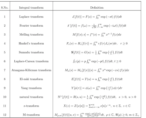
Historically, the origin of the integral transforms can be traced back to the work of P. S. Laplace in
1780s and Joseph Fourier in 1822. In recent years, differential and integral equations have been solved
using many integral transforms ( [1]- [11]). The Laplace transform, and Fourier integral transforms are the
most commonly used in the literature. The Fourier integral transform [12] was named after the French
mathematician Joseph Fourier. Mathematically, Fourier integral transform is defined as:
z[f(t)] =f(ω) = √1
2π Z ∞
−∞
exp (−iωt)f(t)dt. (1.1)
Received 2018-07-27; accepted 2018-10-06; published 2019-03-01.
2010Mathematics Subject Classification. 44A10, 44A15, 44A20, 44A30, 44A35.
Key words and phrases. Shehu transform; Fourier integral transform; Laplace transform; natural transform; Sumudu trans-form; ordinary and partial differential equations.
c
2019 Authors retain the copyrights of their papers, and all open access articles are distributed under the terms of the Creative Commons Attribution License.
The Fourier transform have many applications in physics and engineering processes [13]. The Laplace integral
transform is similar with the Fourier transform and is defined as:
£[f(t)] =F(s) = Z ∞
−∞
exp (−st)f(t)dt. (1.2)
The Laplace transform is highly efficient for solving some class of ordinary and partial differential equations
[14]. By replacing the variable iω with the variable s in Equ.(1.1), the well-known Fourier transform will
become a Laplace transform and the vice-versa. The only difference between the Laplace transform, and the
Fourier transform is that the Laplace transform can be defined for both stable and unstable system while
the Fourier transform can only be defined on a stable system. In mathematical literature, the discrete-time
equivalent of the Laplace transform called z-transform [15] converts a discrete-time signal into a complex
frequency-domain representation. The basic idea of the z-transform was known to Laplace and later it was
re-introduced by the Jewish-Polish mathematician Witold Hurewicz to treat a sampled-data control systems
used with radar in 1947 ( [16]- [17]). In mathematics and signal processing, the bilateral or two-sided
z-transform of a discrete-time signalx[n] is the normal power seriesX(z) which is defined as:
X(z) =Z{x[n]}=
∞
X
n=−∞
x[n]z−n, (1.3)
wherenis an integer andz is in general a complex number [18].
The multiplicative version of the two-sided Laplace transform called the Mellin integral transform is
defined as [19]:
M[f(s);s] =f∗(s) = Z ∞
0
xs−1f(x)dx. (1.4)
The Mellin integral transform is similar with the Laplace transform and Fourier transform and is widely
applied in computer science and number theory due to its invariant property [20,21]. In railway engineering,
the Laplace-Carson transform [22] which is a Laplace-type integral transform named after Pierre Simon
Laplace and John Renshaw Carson is defined as:
ˆ
fC(p) =p
Z ∞
0
exp (−pt)f(t)dt, t≥0. (1.5)
The Laplace-Carson integral transform have many applications in physics and engineering and can easily be
converted into a Mellin deconvolution problem, see [23,24]. In mathematics, the Hankel’s integral transform
[25] which is similar to the Fourier transform was first introduced by the German mathematician Hermann
Hankel and was widely used in physical science and engineering [26]. The Hankel’s transform is defined as:
Fv(s) =Hv[f(r)] =
Z ∞
0
rf(r)Jv(sr)dr, r≥0, (1.6)
In 1993, Watugala introduced a Laplace-like integral transform called the Sumudu integral transform [27].
In recent years, Sumudu transform has been applied to many real-life problems because of its scale and unit
preserving properties ( [28]- [31]). The mathematical definition of the Sumudu transform is given by:
S[f(t)](u) =G(u) = 1 u
Z ∞
0 exp
−t
u
f(t)dt, (1.7)
provided the integral exists for some u. Based on the basic idea of the Laplace and the Sumudu integral
transform, the Elzaki transform was proposed in 2011. The Elzaki transform is closely related with the
Laplace transform, Sumudu transform, and the natural transform. Elzaki transform is defined as [32]:
E[f(t)] =T(u) =u Z ∞
0 exp
−t
u
f(t)dt, (1.8)
provided the integral exists for someu.
The natural transform [33] which is similar to Laplace and Sumudu integral transform was introduced in
2008. In recent years, natural transform was successfully applied to many applications (see [34,35]). The
natural transform is defined by the following integral:
N+[f(t)](s, u) =R(s, u) = 1
u Z ∞
0 exp
−st u
f(t)dt, s >0, u >0, (1.9)
provided the integral exists for some variables uand s. Recently, a new integral transform called the M
-transform which is also similar to natural -transform is introduced by Srivastava et al. in 2015.
Mathemat-ically speaking,M-transform is closely connected with the well-known Laplace transform and the Sumudu
integral transform. M-transform was successfully applied to first order initial-boundary value problem (see
Srivastava et al. [36]). The M-transform is defined as:
Mρ,m[f(t)](u, v) =
Z ∞
0
exp (−ut)f(vt)
(tm+vm)ρ dt, (1.10)
(ρ∈C;<(ρ)≥0, m∈Z+= 1,2,3,· · ·),where bothu∈Candv∈R+ are theM-transform variables.
In 2013, Atangana and Kilicman introduced a novel integral transform called the Abdon-Kilicman integral
transform [37] for solving some differential equations with some kind of singularities. The novel integral
transform is defined as:
Mn(s) =Mn[f(x)](s) =
Z ∞
0
xnexp (−xs)f(x)dx. (1.11)
The Atangana-Kilicman integral becomes Laplace transform whenn= 0. Recently, a Laplace-type integral
transform called the Yang transform ( [38]- [40]) for solving steady heat transfer problems was introduced
in 2016. The integral transform is defined as:
Y[φ(τ)] =φ(ω) = Z ∞
0 exp
−τ
ω
φ(τ)dτ, (1.12)
Due to the rapid development in the physical science and engineering models, there are many other
integral transforms in the literature. However, most of the existing integral transforms have some limitations
and cannot be used directly to solved nonlinear problems or many complex mathematical models. As a
result, many authors became highly interested to come up with the alternative approach for solving many
real-life problems. In 2016, Atangana and Alkaltani introduced a new double integral equation and their
properties based on the Laplace transform and decomposition method. The double integral transform was
successfully applied to second order partial differential equation with singularity called the two-dimensional
Mboctara equation [41]. Recently, Eltayeb applied double Laplace decomposition method to nonlinear partial
differential equations [42]. In 2017, Belgacem el at. extended the applications of the natural and the Sumudu
transforms to fractional diffusion and Stokes fluid flow realms [43].
Motivated by the above-mentioned researches, in this paper we proposed a Laplace-type integral transform
called Shehu transform for solving both ordinary and partial differential equations. The Laplace-type integral
transform converges to Laplace transform when u = 1, and to Yang integral transform whens = 1. The
proposed integral transform is successfully applied to both ordinary and partial differential equations. All
the results obtained in the applications section can easily be verified using the Laplace or Fourier integral
transforms. Throughout this paper, the Shehu transform is denoted by an operatorS[.].
2. Main result
Definition 1. The Shehu transform of the function v(t) of exponential order is defined over the set of
functions,
A=nv(t) :∃ N, η1, η2>0, |v(t)|< Nexp
|t|
ηi
, ift∈(−1)i×[0,∞)o,
by the following integral
S[v(t)] = V(s, u) =
Z ∞
0 exp
−st u
v(t)dt
= lim
α→∞
Z α
0 exp
−st
u
v(t)dt; s >0, u >0. (2.1)
It converges if the limit of the integral exists, and diverges if not.
The inverse Shehu transform is given by
S−1[V(s, u)] =v(t), f or t≥0. (2.2)
Equivalently
v(t) =S−1[V(s, u)] = 1 2πi
Z α+i∞
α−i∞
1 uexp
st
u
where sand uare the Shehu transform variables, andαis a real constant and the integral in Equ.(2.3) is
taken alongs=αin the complex planes=x+iy.
Theorem 1. The sufficient condition for the existence of Shehu transform. If the functionv(t)is
piecewise continues in every finite interval 0≤t≤β and of exponential order αfort > β. Then its Shehu
transform V(s, u)exists.
Proof. For any positive numberβ, we algebraically deduce
Z ∞ 0 exp −st u
v(t)dt= Z β 0 exp −st u
v(t)dt+ Z ∞ β exp −st u
v(t)dt. (2.4)
Since the functionv(t) is piecewise continues in every finite interval 0≤t≤β, then the first integral on the
right hand side exists. Besides, the second integral on the right hand side exists, since the functionv(t) is of
exponential orderαfort > α. To verify this claim, we consider the following case
Z ∞ α exp −st u
v(t)dt ≤ Z ∞ α exp −st u
v(t) dt ≤ Z ∞ 0 exp −st u
|v(t)|dt
≤ Z ∞ α exp −st u
N eexp (βt)dt
= N
Z ∞
α exp
−(s−βu)t
u
dt
= − uN
(s−βu)γlim→∞
exp
−(s−βu)t
u
γ
0
= uN
s−βu.
The proof is complete.
Property 1. Linearity property of Shehu transform. Let the functionsαv(t)and βw(t) be in set A,
then(αv(t) +βw(t))∈A, whereαandβ are nonzero arbitrary constants, and
S[αv(t) +βw(t)] =αS[v(t)] +βS[w(t)]. (2.5)
Proof. Using the Definition 1 of Shehu transform, we get
S[αv(t) +βw(t)] =
Z ∞ 0 exp −st u
(αv(t) +βw(t))dt
= Z ∞ 0 exp −st u
(αv(t))dt+ Z ∞ 0 exp −st u
(βw(t))dt
= α Z ∞ 0 exp −st u
v(t)dt+β Z ∞ 0 exp −st u
w(t)dt
= αu
Z ∞
0
exp (−st)v(ut)dt+βu Z ∞
0
exp (−st)w(ut)dt
The proof is complete.
In particular, using the Definition1 and Property1, we obtain
S[3 cos(t) + 5 sin(2t)] = 3S[cos(t)] + 5S[sin(2t)]
= 3us s2+u2 +
5u2
s2+ (2u)2,
see entries of table 1.
Property 2. Change of scale property of Shehu transform. Let the functionv(βt)be in set A, where
β is an arbitrary constant. Then
S[v(βt)] =
u βV
s
β, u
. (2.6)
Proof. Using the Definition 1 of Shehu transform, we deduce
S[v(βt)] =
Z ∞
0 exp
−st u
v(βt)dt (2.7)
Substitutingη=βtwhich impliest=βη anddt= dηβ in Equ.(2.7) yields
S[v(βt)] = 1
β Z ∞
0 exp
−sη uβ
v(η)dη
= 1
β Z ∞
0 exp
−st
uβ
v(t)dt
= u
β Z ∞
0 exp
−st β
v(ut)dt
= u
βV s
β, u
.
The proof is complete.
Theorem 2. Derivative of Shehu transform. If the functionv(n)(t)is thenthderivative of the function
v(t)∈A with respect to0t0, then its Shehu transform is defined by
S
h
v(n)(t)i= s n
unV(s, u)− n−1
X
k=0
s u
n−(k+1)
v(k)(0). (2.8)
When n=1, 2, and 3 in Equ. (2.8) above, we obtain the following derivatives with respect tot.
S[v0(t)] = s
uV(s, u)−v(0). (2.9)
S[v00(t)] = s 2
u2V(s, u)−
s
uv(0)−v
0(0). (2.10)
S[v000(t)] = s 3
u3V(s, u)−
s2 u2v(0)−
s uv
Proof. Now suppose Equ. (2.8) is true for n=k. Then using Equ. (2.9) and the induction hypothesis, we
deduce
S
h
(v(k)(t))0i = s uS
h
v(k)(t)i−v(k)(0)
= s
u "
sk
ukS[v(t)]− k−1
X
i=0
s u
k−(i+1) v(i)(0)
#
−v(k)(0)
= s
u k+1
S[v(t)]− k
X
i=0
s u
k−i v(i)(0),
which implies that Equ. (2.8) holds forn=k+ 1. By induction hypothesis the proof is complete.
The following important properties are obtain using the Leibniz’s rule
S
∂v(x, t)
∂x = Z ∞ 0 exp −st u
∂v(x, t)
∂x dt= ∂ ∂x Z ∞ 0 exp −st u
v(x, t)dt
= ∂
∂x[V(x, s, u)]⇒S
∂v(x, t) ∂x
= d
dx[V(x, s, u)],
S
∂2v(x, t)
∂x2 = Z ∞ 0 exp −st u
∂2v(x, t)
∂x2 dt=
∂2 ∂x2 Z ∞ 0 exp −st u
v(x, t)dt
= ∂ 2
∂x2[V(x, s, u)]⇒S
∂2v(x, t)
∂x2
= d
2
dx2[V(x, s, u)],
and
S
∂nv(x, t) ∂xn = Z ∞ 0 exp −st u
∂nv(x, t) ∂xn dt=
∂n ∂xn Z ∞ 0 exp −st u
v(x, t)dt
= ∂ n
∂xn[V(x, s, u)]⇒S
∂nv(x, t)
∂xn
= d
n
dxn[V(x, s, u)].
3. Some useful results of Shehu transform
Property 3. Let the function v(t) = 1be in set A. Then its Shehu transform is given by
S[1] = u
s. (3.1)
Proof. Using Equ.(2.1), we deduce
S[1] =
Z ∞ 0 exp −st u
dt=−u
sγlim→∞
exp −st u γ 0 =u s.
This ends the proof.
Property 4. Let the function v(t) =tbe in set A. Then its Shehu transform is given by
S[t] = u 2
Proof. Using the Definition 1 of the Shehu transform and integration by parts, we get
S[t] =
Z ∞ 0 texp −st u
dt=u sγlim→∞
texp −st u γ 0 +u s Z ∞ 0 exp −st u dt
=−u
2
s2 γlim→∞
exp −st u γ 0 = u 2
s2.
Thus the proof ends.
Property 5. Let the function v(t) =tn!n n= 0,1,2.. be in set A. Then its Shehu transform is given by
S
tn n!
=u s
n+1
. (3.3)
Proof. From the Definition 1 of the Shehu transform and integration by parts, we deduce
S[tn] =
Z ∞
0
tnexp −st
u
dt= u sn
Z ∞
0
tn−1exp −st u dt =u 2
s2n(n−1)
Z ∞
0
tn−2exp −st u dt = u 3
s3n(n−1)(n−2)
Z ∞
0
tn−3exp −st u dt =u 4
s4n(n−1)(n−2)(n−3)
Z ∞
0
tn−4exp −st u dt = u 5
s5n(n−1)(n−2)(n−3)(n−4)
Z ∞
0
tn−5exp
−st u
dt=· · ·=n!u s
n+1 .
The proof is completed.
Property 6. Let the function v(t) = Γ(n+1)tn n= 0,1,2,· · · be in set A. Then its Shehu transform is given
by
S
tn
Γ(n+ 1)
=u s
n+1
. (3.4)
The proof of property 6 follows immediately from the previous property 5.
Property 7. Let the function v(t) = exp(αt)be in A. Then its Shehu transform is given by
S[exp(αt)] = u
s−αu. (3.5)
Proof. Using Equ.(2.1), we get
S[exp(αt)] =
Z ∞
0 exp
−(s−αu)t
u
dt
=− u
s−αuγlim→∞
exp
−(s−αu)t
u
γ
0
= u
s−αu.
Property 8. Let the function v(t) =texp(αt)be in set A. Then its Shehu transform is given by
S[texp(αt)] =
u2
(s−αu)2. (3.6)
Proof. Using the Definition 1 of the Shehu transform and integration by parts, we get
S[texp(αt)] =
Z ∞
0
texp
−(s−αu)t
u
dt
=− u
s−αuγlim→∞
texp
−(s−αu)t
u
γ
0
+ u
s−αu Z ∞
0 exp
−(s−αu)t
u
dt
=− u
2
(s−αu)2γlim→∞
exp
−(s−αu)t
u
γ
0
= u
2
(s−αu)2.
The proof is complete.
Property 9. Let the functionv(t) =tnexp(αt)n! n= 0,1,2, ...be in set A. Then its Shehu transform is given
by
S
tnexp(αt) n!
= u
n+1
(s−αu)n+1. (3.7)
Proof. Using the Definition 1 of the Shehu transform and integration by parts, we deduce
S[tnexp(αt)] =
Z ∞
0
tnexp
−(s−αu)t
u
dt
= un
(s−αu) Z ∞
0
tn−1exp
−(s−αu)t
u
dt
= u
2n(n−1)
(s−αu)2
Z ∞
0
tn−2exp
−(s−αu)t
u
dt=· · ·= n! (s−αu)n+1.
Thus the proof is complete.
Property 10. Let the functionv(t) = Γ(n+1)tn exp(αt) n= 0,1,2, ... be in set A. Then its Shehu transform
is given by
S
tnexp(αt)
Γ(n+ 1)
= u
n+1
(s−αu)n+1. (3.8)
The proof of Property 10 follows as a direct consequence of Property 9.
Property 11. Let the function v(t) =sin(αt)be in set A. Then its Shehu transform is given by
S[sin(αt)] =
αu2
Proof. Using the Definition 1 of the Shehu transform and integration by parts, we get
S[sin(αt)] =
Z ∞ 0 exp −st u
sin(αt)dt
=−u
sγlim→∞
exp −st u
sin(αt) γ 0 +uα s Z ∞ 0 exp −st u
cos(αt)dt
= −αu
2
s2 γlim→∞
exp −st u
cos(αt) γ
0
−α
2u2
s2 Z ∞ 0 exp −st u
sin(αt)dt
= αu
2
s2 −
α2u2
s2 Z ∞ 0 exp −st u
sin(αt)dt.
Simplifying the required integrals complete the proof of Property 11.
Property 12. Let the function v(t) = cos(αt)be in set A. Then its Shehu transform is given by
S[cos(αt)] =
us
s2+α2u2. (3.10)
Proof. Using the Definition 1 of the Shehu transform and integration by parts, we deduce
S[cos(αt)] =
Z ∞ 0 exp −st u
cos(αt)dt
=−u
sγlim→∞
exp −st u
cos(αt) γ 0 −αu s Z ∞ 0 exp −st u
sin(αt)dt
= u
s − αu2
s2 γlim→∞
exp −st u
sin(αt) γ
0
−α
2u2
s2 Z ∞ 0 exp −st u
cos(αt)dt
= u
s − α2u2
s2 Z ∞ 0 exp −st u
cos(αt)dt.
Simplifying the required integrals complete the proof of Property 12.
Property 13. Let the function v(t) = sinh(αt)α be in set A. Then its Shehu transform is given by
S
sinh(αt)
α
= u
2
s2−α2u2. (3.11)
Proof. From the Definition 1 of the Shehu transform and integration by parts, we get
S[sinh(αt)] =
Z ∞ 0 exp −st u
sinh(αt)dt
=−u
sγlim→∞
exp −st u
sinh(αt) γ 0 +uα s Z ∞ 0 exp −st u
cosh(αt)dt
= −αu
2
s2 γlim→∞
exp −st u
cos(αt) γ
0 +α
2u2
s2 Z ∞ 0 exp −st u
sinh(αt)dt
= αu
2
s2 +
α2u2
s2 Z ∞ 0 exp −st u
sinh(αt)dt.
Property 14. Let the function v(t) = cosh(αt) be in set A. Then its Shehu transform is given by
S[cosh(αt)] =
us
s2−α2u2. (3.12)
Proof. Applying the Definition 1 of the Shehu transform and integration by parts, we get
S[cosh(αt)] =
Z ∞ 0 exp −st u
cosh(αt)dt
=−u
sγlim→∞
exp −st u
cos(αt) γ 0 +αu s Z ∞ 0 exp −st u
sinh(αt)dt
= u
s − αu2
s γlim→∞
exp −st u
sinh(αt) γ
0 +α
2u2
s2 Z ∞ 0 exp −st u
cos(αt)dt
= u
s + α2u2
s2 Z ∞ 0 exp −st u
cosh(αt)dt.
Collecting the required integrals complete the proof of Property 14.
Property 15. Let the function exp(βt) sin(αt)α be in set A. Then its Shehu transform is given by
S
exp (βt) sin(αt) α
= u
2
(s−βu)2+α2u2. (3.13)
Proof. Using the Definition 1 of the Shehu transform and integration by parts, we deduce
S[exp (βt) sin(αt)] =
Z ∞
0 exp
−(s−βu)
u t
sin(αt)dt
= −u
(s−βu)γlim→∞
exp
−(s−βu)
u t
sin(αt)dt γ
0
+ uα
s−βu Z ∞
0 exp
−(s−βu)
u t
cos(αt)dt
=− u
2α
(s−βu)2γlim→∞
exp
−(s−βu)
u t
cos(αt)dt γ
0
− αu
2α2
(s−βu)2
Z ∞
0 exp
−(s−βu)
u t
sin(αt)dt
= u
2α
(s−βu)2 −
u2α2 (s−βu)2
Z ∞
0 exp
−(s−βu)
u t
sin(αt)dt.
Simplifying the required integrals complete the proof of property 15. This ends the proof.
Property 16. Let the function exp (βt) cos(αt) be in set A. Then its Shehu transform is given by
S[exp (βt) cos(αt)] =
u(s−αu)
Proof. Applying the Definition 1 of the Shehu transform and integration by parts, we get
S[exp (βt) cos(αt)] =
Z ∞
0 exp
−(s−βu)
u t
cos(αt)dt
=− u
s−βuγlim→∞
exp
−(s−βu)
u t
cos(αt)
γ
0
+ αu
s−βu Z ∞
0 exp
−(s−βu)
u t
sin(αt)dt
= u
s−βu+ αu s−βu
Z ∞
0 exp
−(s−βu)
u t
sin(αt)dt
= u
s−βu+ αu2
(s−αu)2γlim→∞
exp
−(s−βu)
u t
sin(αt)
γ
0
− α
2u2
(s−βu)2
Z ∞
0 exp
−(s−βu)
u t
cos(αt)dt
= u
s−βu− α2u2 (s−βu)2
Z ∞
0 exp
−(s−βu)
u t
cos(αt)dt.
Simplifying the required integrals complete the proof of property 16.
Property 17. Let the function exp(βt)β−−exp(αt)α be in set A. Then its Shehu transform is given by
S
exp (αt)
β−α
= u
2
(s−αu)(s−βu). (3.15)
Proof. Using the definition of Shehu transform, we get
S
exp (αt) β−α = u β−α Z ∞ 0 exp −st u
(exp(βt)−exp (αt))dt
= 1
β−α Z ∞
0
e(βu−su )tdt− 1 β−α
Z ∞
0 exp
(αu−s)t
u
dt
= u
(β−α)(βu−s)γlim→∞
exp
−(s−βu)t
u
γ
0
− u
(β−α)(αu−s)γlim→∞
exp
−(s−βu)t
u
γ
0
= − u
(β−α)(βu−s)+
u (β−α)(αu−s)
= −u(αu−s) +u(βu−s) (β−α)(αu−s)(βu−s)=
u2
(s−αu)(s−βu).
The proof is complete.
Property 18. Let the function βexp(βt)β−−ααexp(αt) be in set A. Then its Shehu transform is given by:
S
βexp (βt)−αexp (αt)
β−α
= us
Proof:
Using the definition of Shehu transform, we get
S
βexp (βt)−αexp (αt)
β−α
= 1
β−α Z ∞
0 exp
−st
u
(βexp (βt)−αexp (αt))dt
= β
β−α Z ∞
0 exp
(βu
−s)
u t
dt− α
β−α Z ∞
0 exp
(αu
−s)t u
dt
= uβ
(β−α)(βu−s)γlim→∞
exp
−(s−βu)t
u
γ
0
− uα
(β−α)(αu−s)γlim→∞
exp
−(s−αu)t
u
γ
0
= − uβ
(β−α)(βu−s)+
uα (β−α)(αu−s)
= −uβ(αu−s) +uα(βu−s) (β−α)(αu−s)(βu−s) =
us
(s−αu)(s−βu).
This ends the proof.
More properties of the Shehu transform and their converges to the natural transform, the Sumudu
trans-form, and the Laplace transform are presented in table 1. The comprehensive summary of Shehu transform
properties are presented in table 2.
4. Applications
In this section, the applications of the proposed transform are presented. The simplicity, efficiency and
high accuracy of the Shehu transform are clearly illustrated.
Example 1. Consider the following first order ordinary differential equation
dv(t)
dt +v(t) = 0, (4.1)
subject to the initial condition
v(0) = 1. (4.2)
Applying the Shehu transform on both sides of Equ. (4.1), we get
s
uV(s, u)−v(0) +V(s, u) = 0. (4.3)
Substituting the given initial condition and simplifying, we deduce
V(s, u) = u
s+u (4.4)
Taking the inverse Shehu transform of Equ. (4.4), yields
Example 2. Consider the following second order ordinary differential equation
d2v(t) dt2 +
dv(t)
dt = 1 (4.6)
subject to the initial conditions
v(0) = 0, dv(0)
dt = 0. (4.7)
Applying the Shehu transform on both sides of Equ. (4.6), we obtain
s2
u2V(s, u)−
s
uv(0)−v
0(0) + s
uV(s, u)−v(0) = u
s. (4.8)
Substituting the given initial conditions and simplifying, we deduce
V(s, u) =−u
s + u2
s2 +
u
s+u. (4.9)
Taking the inverse Shehu transform of Equ. (4.9), we get
v(t) =−1 +t+ exp(−t). (4.10)
Example 3. Consider the following second nonhomogeneous order ordinary differential equation
d2v(t) dt2 −3
dv(t)
dt + 2v(t) = exp(3t). (4.11)
subject to the initial conditions
v(0) = 1, dv(0)
dt = 0. (4.12)
Applying the Shehu transform on both sides of Equ. (4.11), yields
s2
u2V(s, u)−
s
uv(0)−v
0(0)−3s
uV(s, u)−v(0)
+ 2V(s, u) = u
s−3u. (4.13)
Substituting the given initial conditions and simplifying, we obtain
V(s, u) =5 2
u (s−u)−2
u s−2u+
1 2
u
(s−3u). (4.14)
Taking the inverse Shehu transform of Equ. (4.14), we get
v(t) =5
2exp(t)−2 exp(2t) + 1
2exp(3t). (4.15)
Example 4. Consider the following ordinary differential equation
d2v(t) dt2 + 2
dv(t)
dt + 5v(t) = exp(−t) sin(t). (4.16)
subject to the initial conditions
v(0) = 0, dv(0)
dt = 1. (4.17)
Applying the Shehu transform on both sides of Equ. (4.16), we get
s2
u2V(s, u)−
s
uv(0)−v
0(0) + 2s
uV(s, u)− s uv(0)
+ 5V(s, u) = u 2
Substituting the given initial conditions and simplifying, we get
V(s, u) =1 3
u2
((s+u)2+u2)+ 2 3
u2
((s+u)2+ (2u)2) (4.19)
Taking the inverse Shehu transform of Equ. (4.19), we get
v(t) =1
3exp(−t) sin(t) + 2
3exp(−t) sin(2t). (4.20)
Example 5. Consider the following homogeneous partial differential equation
∂v(x, t) ∂t =
∂2v(x, t)
∂x2 (4.21)
subject to the boundary and initial conditions
v(0, t) = 0, v(1, t) = 0, v(x,0) = 3sin(2πx). (4.22)
Applying the Shehu transform on both sides of Equ. (4.21), we get
s
uV(x, s, u)−v(x,0) =
d2V(x, s, u)
dx2 . (4.23)
Substituting the given initial condition and simplifying, we get
d2V(x, s, u) dx2 −
s
uV(x, s, u) =−3sin(2πx). (4.24)
The general solution of Equ. (4.24) can be written as
V(x, s, u) =Vh(x, s, u) +Vp(x, s, u), (4.25)
whereVh(x, s, u) is the solution of the homogeneous part which is given by
Vh(x, s, u) =α1exp
r s ux
+α2exp
−
r s ux
, (4.26)
andVp(x, s, u) is the solution of the nonhomogeneous part which is given by
Vp(x, s, u) =β1sin(2πx) +β2cos(2πx). (4.27)
Applying the boundary conditions on Equ. (4.26), we get
α1+α2= 0 and α1exp
rs
u
+α2exp
−
r s u
= 0⇒Vh(x, s, u) = 0,
sinceα1=α2= 0.
Using the method of undetermined coefficients on the nonhomogeneous part, we get
Vp(x, s, u) = 3u
s+ 4π2usin(2πx), (4.28)
Since,β1= s+4π3u2u, and β2= 0.
Then Equ. (4.25) will become
V(x, s, u) = 3u
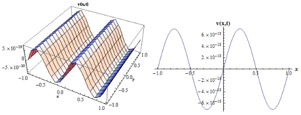
Taking the inverse Shehu transform of Equ. (4.29), we get
v(x, t) = 3 exp(−4π2t) sin(2πx). (4.30)
Figure 1. 3D and 2D surfaces of the analytical solution of Equ. (4.21) in the ranges −1 < x < 1, and
−1< t <1, whent= 1.
Example 6. Consider the following nonhomogeneous partial differential equation
∂2v(x, t)
∂t2 =β 2∂
2v(x, t)
∂x2 + sin(πx) (4.31)
subject to the boundary and initial conditions
v(0, t) = 0, v(1, t) = 0, v(x,0) = 0, ∂v(x,0)
∂t = 0, β
2= 1. (4.32)
Applying the Shehu transform on both sides of Equ. (4.31), we get
s2
u2V(x, s, u)−
s
uv(x,0)−v
0(x,0) = d2V(x, s, u)
dx2 +
u
s sin(πx). (4.33)
Substituting the given initial condition and simplifying, we get
d2V(x, s, u)
dx2 −
s2
u2V(x, s, u) =−
u
ssin(πx). (4.34)
The general solution of Equ. (4.34) can be written as
V(x, s, u) =Vh(x, s, u) +Vp(x, s, u), (4.35)
whereVh(x, s, u) is the solution of the homogeneous part which is given by
Vh(x, s, u) =λ1exp
s ux
+λ2exp
−s
ux
, (4.36)
andVp(x, s, u) is the solution of the nonhomogeneous part which is given by
Vp(x, s, u) =η1sin(πx) +η2cos(πx). (4.37)
Applying the boundary conditions on Equ. (4.36), we deduce
λ1+λ2= 0 and λ1exp
s u
+λ2exp
−s
u
sinceλ1=λ2= 0.
Using the method of undetermined coefficients on the nonhomogeneous part, we get
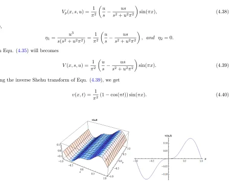
Vp(x, s, u) = 1 π2
u
s − us s2+u2π2
sin(πx), (4.38)
since,
η1=
u3
s(s2+u2π2) = 1 π2
u
s − us s2+u2π2
, and η2= 0.
Then Equ. (4.35) will becomes
V(x, s, u) = 1 π2
u
s − us s2+u2π2
sin(πx). (4.39)
Taking the inverse Shehu transform of Equ. (4.39), we get
v(x, t) = 1
π2(1−cos(πt)) sin(πx). (4.40)
Figure 2. 3D and 2D surfaces of the analytical solution of Equ. (4.31) in the ranges −1 < x < 1, and
−1< t <1.
5. Conclusion
We introduced an efficient Laplace-type integral transform called the Shehu transform for solving both
ordinary and partial differential equations. We presented its existence and inverse transform. We presented
some useful properties and their applications for solving ordinary and partial differential equations. We
provide a comprehensive list of the Laplace transform, Sumudu transform, and the natural transform in
table 1 to show their mutual relationship with the Shehu transform. Finally, based on the mathematical
formulations, simplicity and the findings of the proposed integral transform, we conclude that it is highly
efficient because of the following advantages:
• It is a generalization of the Laplace and the Sumudu integral transforms.
• The Laplace-type integral transform become Laplace transform when the variable u= 1 and the
Yang integral transform when the variables= 1.
• It can easily be applied directly to some class of ordinary and the partial differential equations as
demonstrated in the application section.
• For advanced research in physical science and engineering, the proposed integral transform can be
considered a stepping-stone to the Sumudu transform, the natural transform, the Elzaki transform,
and the Laplace transform.
6. ACKNOWLEDGEMENTS
The authors are highly grateful to the editor’s and the anonymous referees’ for their useful comments and
suggestions in this paper. This research is partially supported by the National Natural Science Foundations
of China under Grants No. 11571206. The first author also acknowledges the financial support of Chinese
Scholarship Council (CSC) in Shandong University with grand (CSC No: 2017GXZ025381).
References
[1] H.A. Agwa, F.M. Ali, A. Kilicman, A new integral transform on time scales and its applications, Adv. Difference Equ., 60(2012), 1–14.
[2] C. Ahrendt, The Laplace transform on time scales, Pan. Amer. Math. J., 19(2009), 1–36.
[3] A. Atangana, A note on the triple Laplace transform and its applications to some kind of third-order differential equation, Abstr. Appl. Anal., 2013(2013), Article ID 769102, 1–10.
[4] H.M. Srivastava, A.K. Golmankhaneh, D. Baleanu, X.Y. Yang, Local fractional Sumudu transform with applications to IVPs on Cantor sets, Abstr. Appl. Anal., 2014(2014), Article ID 620529, 1–7.
[5] G. Dattoli, M. R. Martinelli, P. E. Ricci, On new families of integral transforms for the solution of partial differential equations, Integral Transforms Spec. Funct., 8(2005), 661–667.
[6] H. Bulut, H.M. Baskonus, and F.B.M. Belgacem, The analytical solution of some fractional ordinary differential equations by the Sumudu transform method, Abstr. Appl. Anal., 2013(2013), Article ID 203875, 1–6.
[7] S.Weerakoon, The Sumudu transform and the Laplace transform: reply, Int. J. Math. Educ. Sci. Technol., 28(1997), 159–160.
[8] D. Albayrak, S.D. Purohit, and F. U¸car, Certain inversion and representation formulas for q-sumudu transforms, Hacet. J. Math. Stat., 43(2014), 699–713.
[9] S. Weerakoon, Application of Sumudu transform to partial differential equations, Int. J. Math. Educ. Sci. Technol., 25(1994), 277–283.
[10] X.Y. Yang, Y. yang, C. Cattani, and M. Zhu, A new technique for solving 1-D Burgers equation, Thermal Science, 21(2017), S129–S136.
[11] A. Kilicman, H. Eltayeb, On new integral transform and differential equations, J. Math. Probl. Eng, 2010(2010), Article ID: 463579, 1–13.
[14] R. Murray, Spiegel. Theory and problems of Laplace transform. New York, USA: Schaum’s Outline Series, McGraw–Hill, (1965).
[15] L. Debnath, D. Bhatta.. Integral transform and their applications. CRC Press, New York, NY, USA (2010).
[16] B. Davies, Integral transforms and their applications, Texts in Applied Mathematics, Springer, New York, NY, USA, (2002).
[17] E.I. Jury, Theory and applications of the z-transform Method, John Wiley and Sons, New York, NY,USA, (1964). [18] K. Liu, R.J. Hu, C. Cattani, G.N. Xie, X.J. Yang, and Y. Zhao, Local fractional z-transforms with applications to signals
on Cantor sets, Abstr. Appl. Anal., 2014(2014),Article ID: 638648, 1–6.
[19] P.M. Morse, H. Feshbach, Methods of theoretical physics, McGraw-Hill, New York, (1953), 484–485.
[20] P. Flajolet, X. Gourdon, and P. Dumas, Mellin transforms and asymptotics: harmonic sums, Theor. Comput. Sci., 144(1995), 3–58.
[21] C. Donolato, Analytical and numerical inversion of the Laplace-Carson transform by a differential method, Comput. Phys. Commun., 145(2002), 298–309.
[22] A.M. Makarov, Application of the Laplace-Carson method of integral transformation to the theory of unsteady visco-plastic flows, J. Engrg. Phys. Thermophys 19(1970), 94–99.
[23] E. Sjntoft, A straightforward deconvolution method for use in small computers, Nucl. Instrum. Methods, 163(1979), 519–522.
[24] A.S. Vasudeva Murthy, A note on the differential inversion method of Hohlfield et al., SIAM J. Appl. Math., 55(1995), 712–722.
[25] I.N. Sneddon, The Use of integral transform, McGraw-Hill, New York, (1972).
[26] K. Xie, Y. Wanga, K. Wang, and X. Cai, Application of Hankel transforms to boundary value problems of water flow due to a circular source, Appl. Math. Comput., 216(2010), 1469–1477.
[27] Watugala GK. Sumudu transform–a new integral transform to solve differential equations and control engineering problems. Math. Engg. Indust., 6(1998), 319–329.
[28] M.A. Asiru, Sumudu transform and solution of integral equations of convolution type, Int. J. Math. Edu. Sci. Tech., 33(2002), 944–949.
[29] F.B.M. Belgacem, S.L. Kalla, A.A. Karaballi, Analytical investigations of the Sumudu transform and applications to integral production equations, Math. Probl. Engg., 3(2003), 103-118.
[30] F.B.M. Belgacem, A.A. Karaballi, Sumudu transform fundamental properties, investigations and applications. J. Appl. Math. Stoch. Anal., 2006(2006), Article ID 91083, 1–23.
[31] H. ELtayeh and A. kilicman, On Some applications of a new integral transform, Int. J. Math. Anal., 4(2010), 123–132. [32] T.M. Elzaki. The new integral transform ”Elzaki transform”. Glob. J. Pure Appl. Math., 7(2011), 57–64.
[33] Z.H. Khan, W.A. Khan, N-transform-properties and applications. NUST J. Engg. Sci., 1(2008), 127–133. [34] F.B.M. Belgacem, R. Silambarasan, Theory of natural transform. Math. Engg. Sci. Aeros., 3(2012), 99–124.
[35] F.B.M. Belgacem, R. Silambarasan, Advances in the natural transform. AIP Conference Proceedings; 1493 January 2012; USA: American Institute of Physics. (2012), 106–110.
[36] H.M. Srivastava, Minjie Luo, R.K.Raina, A new integral transform and its applications, Acta Math. Sci., 35(2015), 1386–1400.
[38] X.J. Yang, A new integral transform method for solving steady heat-transfer problem, Thermal Science, 20(2016), S639–S642.
[39] X.J. Yang, A new integral transform operator for solving the heat-diffusion problem, Appl. Math. Lett., 64(2017), 193–197. [40] Y.X. Jun, F. Gao , A new technology for solving diffusion and heat equations, Thermal Science, 21(2017), 133–140. [41] A. Atangana, B.S.T. Alkaltani, A novel double integral transform and its applications, J. Nonlinear Sci. Appl., 9(2016),
424–434.
[42] H. Eltayeb, A note on double Laplace decomposition method and nonlinear partial differential equations, New Trends Math. Sci., 5(2017), 156–164.
Appendix
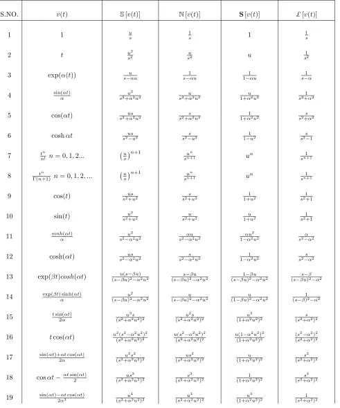
Table 1: Here we present a comprehensive list of the Shehu transform of some special functions and their
relationship with the natural transformN[v(t)], the Sumudu transformS[v(t)], and the Laplace transform.
S.NO. v(t) S[v(t)] N[v(t)] S[v(t)] £[v(t)]
1 1 us 1s 1 1s
2 t us22
u
s2 u
1 s2
3 exp(α(t)) s−uαu s−1αu 1−1αu s−1α
4 sin(αt)α u2
s2+α2u2
u s2+α2u2
u 1+α2u2
1 s2+α2
5 cos(αt) s2+αus2u2
s s2+α2u2
1 1+α2u2
s s2+α2
6 coshαt s2us−u2
s s2−u2
1 1−u2
s s2−1
7 tn
n! n= 0,1,2...
u s
n+1 un
sn+1 u
n 1
sn+1
8 Γ(n+1)tn n= 0,1,2, ... usn+1 un
sn+1 un
1 sn+1
9 cos(t) s2us+u2
s s2+u2
1 1+u2
1 s2+1
10 sin(t) u2
s2+u2
u s2+u2
u 1+u2
1 s2+1
11 sinh(αt)α s2−uα22u2
αu s2−α2u2
αu2
1−α2u2
α s2−α2
12 cosh(αt) s2−usα2u2
s s2−α2u2
1 1−α2u2
s s2−α2
13 exp(βt)cosh(αt) (s−u(sβu)−2βu)−α2u2
s−βu (s−βu)2−α2u2
1−βu (s−βu)2−α2u2
s−β (s−βu)2−α2
14 exp(βt) sinh(αt)α (s−βu)u22−α2u2
u (s−βu)2−α2u2
u (1−βu)2−α2u2
1 (s−β)2−α2
15 tsin(αt)2α u3s
(s2+α2u2)2
u2s (s2+α2u2)2
u3 (1+α2u2)2
s (s2+α2)2
16 tcos(αt) u(s2(s2+α2−α22uu2)22)2
u(s2−α2u2)2
(s2+α2u2)2
u(1−α2u2)2
(1+α2u2)2
(s2−α2)2
(s2+α2)2
17 sin(αt)+αt2αcos(αt) (s2+αu2s22u2)2
us2
(s2+α2u2)2
u (1+α2u2)2
s2
(s2+α2)2
18 cosαt−αtsin(αt)2 us3
(s2+α2u2)2
s3 (s2+α2u2)2
1 (1+α2u2)2
s3 (s2+α2)2
19 sin(αt)−2ααt3cos(αt)
u4
(s2+α2u2)2
u3
(s2+α2u2)2
u3
(1+α2u2)2
20 tsinh(αt) +tcosh(αt) (s−uαu)2 2
u (s−αu)2
u2
(1−αu)2
1 (s−α)2
21 tsinh(αt)2α (s2−uα32su2)2
u2s
(s2−α2u2)2
u2
(1−α2u2)2
s (s2−α2)2
22 Si(αt) (Sine integral) u stan
−1 αu s
1
stan −1 αu
s
tan−1u√α2 1 stan
−1 α s
23 Ci(αt) (Cosine integral) −u 2slog
s2+α2
α2
−1 2slog
s2+α2u2
α2u2
−1 2log
α2u2+1
α2u2
−1 2slog
s2+α2
α2
24 Ei(αt) (Exp. integral) −u slog
αu−s αu
−1 slog
αu−s αu
log αuαu−1
−1 slog
α−s α
25 (3−α2t2) sin(αt)8α5−3αtcos(αt)
u6 (s2+α2u2)3
u5 (s2+α2u2)3
u5 (1+α2u2)3
1 (s2+α2)3
26 (3−α2t2) sin(αt)+5αt8α cos(αt) (s2+αu2s24u2)3
us4
(s2+α2u2)3
u (1+α2u2)3
s4
(s2+α2)3
27 (8−α2t2) cos(αt)8 −7αtsin(αt) (s2+αus25u2)3
s5
(s2+α2u2)3
1 (1+α2u2)3
s5
(s2+α2)3
28 t2sin(αt)2α u4(s(3s2+α2−2αu22u)32)
u3(3s2−α2u3)
(s2+α2u2)3
u3(−3+α2u2)
(1+α2u2)3
(3s2−α2)
(s2+α2)3
29 t2cos(αt)2 u3(s(s23+α−3α2u22u)23s)
u2(s3−3α2u2s)
(s2+α2u2)3
u2(1−3α2u2)
(1+α2u2)3
(s3−3α2s)
(s2+α2)3
30 t3sin(αt)24α su(s25+α(s−2αu)u2)42
su4(s−αu)2 (s2+α2u2)4
u4(1−αu)2 (1+α2u2)4
s(s−α)2 (s2+α2)4
31 exp(αt)α−−exp(βt)β α6=β u2 (s−αu)(s−βu)
u (s−αu)(s−βu)
u (1−βu)(1−αu)
1 (s−β)(s−α)
32 αexp(αt)α−−ββexp(βt) α6=β (s−βu)(sus−αu) (s−βu)(ss −αu) (1−βu)(11 −αu) (s−β)(ss −α)
33 I0(αt) √s2−uα2u2
1 √
s2−α2u2
1 √
1−α2u2
1 √
s2−α2
34 δ(t−α) uexp −uαs 1
uexp −αs u 1 uexp −α u
exp(−αs)
35 J0(αt) √s2+αu 2u2
1 √
s2+α2u2
1 √
1+α2u2
1 √
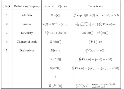
Table 2: General properties of Shehu transform
S.NO. Definition/Property S[v(t)] =V(s, u) Transforms
1 Definition S[v(t)] R∞
0 exp −st
u
v(t)dt; s >0, u >0
2 Inverse v(t) =S−1[V(s, u)] 2πi1
Rα+i∞
α−i∞ 1 uexp
st u
V(s, u)ds
3 Linearity S[αv(t) +βw(t)] αS[v(t)] +βS[w(t)]
4 Change of scale S[v(αt)] u
αV s α, u
5 Derivatives S[v0(t)] usV(s, u)−v(0)
S[v00(t)] s 2
u2V(s, u)−
s
uv(0)−v 0(0)
S[v000(t)] s 3
u3V(s, u)−
s2
u2v(0)−
s uv
0(0)−v00(0)
.. .
Sv(n)(t) s
n
unV(s, u)− Pn−1
k=0 s u
Table 3: Summary of some integral transform and their definitions
S.No. Integral transform Definition
1 Laplace transform £[f(t)] =F(s) =R∞
0 exp (−st)f(t)dt
2 Fourier transform z[f(t)] =f(ω) =√1 2π
R∞
−∞exp (−iωt)f(t)dt
3 Melling transform M[f(s);s] =f∗(s) =R0∞xs−1f(x)dx
4 Hankel’s transform Fv(s) =Hv[f(r)] =
R∞
0 rf(r)Jv(sr)dr, r≥0
5 Sumudu transform S[f(t)] =G(u) =u1R∞
0 exp −t
u
f(t)dt
6 Laplace-Carson transform fˆC(p) =p
R∞
0 exp (−pt)f(t)dt, t≥0
7 Atangana-Kilicman transform Mn(s) =Mn[f(x)](s) =
R∞
0 x
nexp (−xs)f(x)dx
8 El-zaki transform E[f(t)] =T(u) =uR∞
0 exp −t
u
f(t)dt
9 Yang transform Y[φ(τ)] =φ(ω) =R∞
0 exp −τ
ω
φ(τ)dτ
10 natural transform N+[f(t)] =R(s, u) = 1 u
R∞
0 exp −st
u
f(t)dt, s >0, u >0
11 z-transform X(z) =Z{x[n]}=P∞
n=−∞x[n]z− n, n∈
Z, z∈C
12 M-transform Mρ,m[f(t)](u, v) =
R∞
0
exp(−ut)f(vt)