Anomaly Detection Using Autoencoders in High Performance Computing Systems

The Thirty-First AAAI Conference on Innovative Applications of Artificial Intelligence (IAAI-19)

Anomaly Detection Using Autoencoders in High Performance Computing Systems

Andrea Borghesi,

Andrea Bartolini,

Michele Lombardi,

Michela Milano,

Luca Benini

[email protected], [email protected], [email protected], [email protected], [email protected]

Abstract

Anomaly detection in supercomputers is a very difficult prob-lem due to the big scale of the systems and the high num-ber of components. The current state of the art for automated anomaly detection employs Machine Learning methods or statistical regression models in a supervised fashion, mean-ing that the detection tool is trained to distmean-inguish among a fixed set of behaviour classes (healthy and unhealthy states). We propose a novel approach for anomaly detection in High Performance Computing systems based on a Machine (Deep) Learning technique, namely a type of neural network called

autoencoder. The key idea is to train a set of autoencoders to learn the normal (healthy) behaviour of the supercom-puter nodes and, after training, use them to identify abnormal conditions. This is different from previous approaches which where based on learning the abnormal condition, for which there are much smaller datasets (since it is very hard to iden-tify them to begin with).

We test our approach on a real supercomputer equipped with a fine-grained, scalable monitoring infrastructure that can provide large amount of data to characterize the system be-haviour. The results are extremely promising: after the train-ing phase to learn the normal system behaviour, our method is capable of detecting anomalies that have never been seen be-fore with a very good accuracy (values ranging between 88% and 96%).

Introduction

High Performance Computing (HPC) systems are complex machines with many components that must operate concur-rently at the best of their theoretical performance. In reality, many factors can degrade the performance of a HPC system: hardware can break, the applications may enter undesired and unexpected states, components can be wrongly config-ured. A critical aspect of modern and future supercomput-ers is the capability of detecting faulty conditions stemming from the improper behaviour of one or multiple parts. This issue is relevant not only for scientific computing systems but also in data centers and clouds providers, whose busi-ness strongly relies on the availability of their web services. For instance, Amazon in 2016 would have lost 15M$ for just an hour of out of service (Hennessy and Patterson 2011). An

Copyright c2019, Association for the Advancement of Artificial Intelligence (www.aaai.org). All rights reserved.

automated process for anomaly detection would be a great improvement for current HPC systems, and it will probably be a necessity for future Exascale supercomputers.

Nowadays, monitoring infrastructures are available in many HPC systems and data centers, used to gather data about the state of the systems and their components thanks to a large variety of measurement sensors. Given the del-uge of data originating from a monitoring framework, real-time identification of problems and undesired situations is a daunting task for system administrators. The growing scale of HPC systems will only make this task even more difficult. In this paper we present a novel approach to deal with this is-sue, relying on a fine-grain monitoring framework and on an autonomous anomaly detection method that uses Machine Learning (ML) techniques.

Automated anomaly detection is still a relatively unex-plored area in the HPC field. The current state-of-the-art re-lies onsupervised(Mitchell 1999) ML methods that learn to distinguish between healthy and faulty states after a training phase during which the supercomputer must be subjected to different conditions, namely the behaviour classes to be identified, for example normal behaviour and a set of anoma-lies. With this scheme, the anomaly detector learns to clas-sify different classes usinglabeledtraining data.

re-quire any label and it is referred to asunsupervised(Mitchell 1999) learning. In this case the data set contains only the fea-tures describing the system state and no labels; the learning algorithm learns useful properties about the structure of the dataset. To address the issue, we propose an anomaly detec-tion method less dependent on labeled data; to be precise, our approach belongs to thesemi-supervisedbranch of ML, which combines the two methodologies described before. Our idea is to use autoencoders (Goodfellow et al. 2016) to learn the normal behaviour of supercomputer nodes and then to use them to detect abnormal states. In our method we require labels during the pre-processing phase because we need to obtain a data set containing only normal conditions. After this “normal” data set has been obtained the training of the ML model proceeds in unsupervised fashion, without the need of labels. A critical advantage of our method is that it will be able to identify faulty conditions even though these have not been encountered earlier during the training phase. With our method we do not need to inject anomalies during the training phase (possibly not feasible in a production sys-tem) and we do not require system logs or changes to the standard supercomputer users’ work flow.

The main contributions of our approach are: 1) a very precise anomaly detection rate (up to 88%-96% accuracy); 2) identification of new types of anomalies unseen during the initial training phase (thanks to its semi-supervised na-ture); 3) no need for large amount of labeled data. To demon-strate the feasibility of our approach we consider a real su-percomputer hosted by the Italian inter-universities consor-tium CINECA (CIN ). We use historical data collected with an integrated monitoring system to train our autoencoders and then we test them by injecting anomalies in a subset of the computing nodes; the experimental results show how this approach can distinguish between normal and anoma-lous states with a very high level of accuracy.

Related Works

Anomaly Detection in HPC Systems

Tuncer et al. (Tuncer et al. 2017) deal with the problem of diagnosing performance variations in HPC systems. The ap-proach is based on the collection of several measurements gathered by a monitoring infrastructure; from these mea-sures, a set of statistical features describing the state of the supercomputer is extracted. The authors then train differ-ent ML algorithms to classify the behaviour of the super-computer using the statistical features previously mentioned. Unfortunately the authors propose a supervised approach which is not perfectly suited for the HPC context (as dis-cussed previously).

Baseman et al. (Baseman et al. 2016) propose a similar method for anomaly detection in HPC systems. They apply a general statistical technique calledclassifier-adjusted den-sity estimation(CADE) to the HPC context. CADE relies on the observation that combining a uniform density estimate and the probabilistic output of a classifier results in an accu-rate density estimator. First they extract temporal relational features and their gradients from the sensor data. Then they use both real and artificially generated data (thanks to

den-sity estimation) to train a supervised classifier, specifically a Random Forest classifier, in order to rank each data point depending on its “anomalousness”. Again, the main limit of this work is to be based on a supervised approach.

Dani et al. (Dani, Doreau, and Alt 2017) present an un-supervised approach for anomaly detection in HPC. Their work is remarkably different from our approach since they do not rely on a monitoring infrastructure but consider only the console logs generated by computing nodes. The goal of the method is to distinguish log messages regarding faulty situations from logs generated by nodes in normal condi-tion; in order to do so clustering methods (k-means) are used. This work focuses on faults that can be recognized by a node itself and recorded in a log message, thus greatly lim-iting the class of detectable anomalies. Conversely, in our approach we infer anomalies using simply the data collected by a monitoring infrastructure, without requiring a mecha-nism to identify anomalies on the nodes.

Anomaly Detection with Deep Learning

Approaches

Although not yet applied to the HPC field, Deep Learning based approaches for anomaly detection have been stud-ied in other areas (Kwon et al. 2017; Kiran, Thomas, and Parakkal 2018), especially in recent years.

Lv et al. (Lv et al. 2016) propose a deep learning based algorithm for fault diagnosis in chemical production sys-tems. The proposed method is capable of real time detec-tion and classificadetec-tion and, moreover, it can do the diagnosis online. Nevertheless, their approach is supervised and thus it definitely differs from ours. Lee et al. (Lee, Cheon, and Kim 2017) introduce a convolutional neural network (CNN) model for fault identification and classification in semicon-ductor manufacturing processes. This method makes it pos-sible to locate the variable and time information that repre-sents process faults.

Costa et al. (Costa, Angelov, and Guedes 2015) describe a fully unsupervised algorithm for real-time detection of faults in industrial plants. The algorithm relies on the identifica-tion of a set of features that are then used to learn the normal behaviour of the plant, expressing it as a probability den-sity estimation. The online classifier then uses the distance from the normal distribution to classify new data samples. The model is unsupervised and it can handle unseen types of anomalies. However, the approach is specifically targeted at plants for industrial process control and thus not well suited for our HPC system case. Particularly, a relatively small set of features is considered w.r.t. to the hundreds (thousands) of metrics found in a supercomputer.

Ince et al. (Ince et al. 2016) discuss a CNN-based method for electrical motor fault detection; their method can work directly on the raw measurement data, with no preprocess-ing. The neural network combines feature extraction and classification, but proceeds in a supervised manner.

Data Collection

and thus describes the state of a supercomputer. To test our approach we take advantage of a supercomputer with an integrated monitoring infrastructure able to handle large amounts of data coming from several different sources. Our target system is D.A.V.I.D.E.(Ahmad et al. 2017), an energy efficient supercomputer developed by E4 Computer Engi-neering (e4 ) and hosted by CINECA in Bologna, Italy. It is composed by 45 nodes with a total peak performance of 990 TFlops and an estimated power consumption of less than 2 kW per node. Each node hosts two IBM POWER8 Pro-cessors with NVIDIA NVLink and four Tesla P100 GPUs. The system was ranked #440 in TOP500 (Dongarra, Meuer, and Strohmaier 1994) and #18 in GREEN500 (Feng and Cameron 2007) in November 2017 list.

The data collection infrastructure deployed in D.A.V.I.D.E. is called Examon and has been pre-sented in previous works (Beneventi et al. 2017; Bartolini et al. 2018). Examon is a fine-grained, lightweight and scalable monitoring infrastructure for Exascale su-percomputers. The data coming from heterogeneous data sources is gathered in an integrated and uniform repository, making it very easy to create data sets providing a holistic view of the supercomputer and thus describing the system state. The main components of the Examon framework are a set of agents running outside the computing nodes, but tightly coupled with them. These agents monitor the power consumption of each computing node at the plug as well as performance and utilization metrics. The monitored values are sent to a data management backbone, through a communication layer based on the open-source MQTT protocol, a TCP/IP protocol designed for low bandwidth and high latency networks, with minimal resource demands. Since there are limitations on the storage space available for the monitoring infrastructure, it is impossible to store the raw data. The solution adopted in D.A.V.I.D.E. was to discard the fine-grained data older than a week and to pre-serve indefinitely job information and coarse-grained data (long term storage, around 6GB after 7 months of activity). For this paper, we work with the coarse-grained data aggre-gated in 5-minutes long intervals. Furthermore, we focused on a subset of the data collected by Examon; for each node we have 166 metrics (ourfeatures), i.e. core loads, tempera-tures, fan speed, power consumptions, etc.

The Autoencoder-Based Approach

We aim at detecting anomalies that happen at the node-level. Currently, we focus on single nodes. We create a set of sep-arate autoencoder models, one for each node in the system. Each model is trained to learn the normal behaviour of the corresponding node and to be activated if anomalous con-ditions are measured. If an autoencoder can learn the corre-lations between the set of measurements (features) that de-scribe the state of a supercomputer, then it can consequently notice changes in these correlations that indicate an abnor-mal state. Under norabnor-mal operating conditions these features are linked by specific relations (i.e. the power consumption of a core is directly related to the workload and temperature to the power and frequency). We hypothesize that these

cor-relations will be perturbed if the system enters in an anoma-lous state.

Thereconstruction erroris the element we use to detect anomalies. An autoencoder can be trained to minimize this error. In doing so, it learns the relationships among the fea-tures of the input set. If we feed a trained autoencoder with data not seen during the training phase, it should reproduce the new input with good fidelity, at least if the new data re-semble the data used for the training. If this is not the case, the autoencoder cannot correctly reconstruct the input and the error will be greater. We propose to detect anomalies by observing the magnitude of the reconstruction error.

All autoencoders have the same structure. We opted for a fairly simple structure composed by three layers: I) an input layer with as many neurons as the number of features (166), II) a densely connected intermediate sparse layer (Ranzato, Boureau, and Lecun 2008) with 1660 neurons (ten times the number of features) with Rectified Linear Units (ReLu) as activation functions and a L1 norm regularizer (Goodfellow et al. 2016), III) a final dense output layer with 166 neurons with linear activations. This network was obtained after an empirical evaluation, after having experimented with differ-ent topologies and parameter configurations. To summarize, our methodology has the following steps: 1) create an au-toencoder for each computing node in the supercomputer; 2) train the autoencoders using data collected during normal operating conditions; 3) identify anomalies in new data us-ing the reconstruction error obtained by the autoencoders.

Experimental Evaluation

In every HPC system there are multiple possible sources of anomalies and fault conditions, ranging from hardware faults to software errors. In this paper we verify the proposed ap-proach on a type of anomaly that easily arises in real sys-tems and happens at the level of single nodes, namely mis-configuration. More precisely, we consider the misconfigura-tion of the frequency governor of a computing node. Modern Linux systems allow to specify different policies regulating the clock speed of the CPUs, thanks to kernel-level drivers referred as frequency governors (Brodowski and Golde 2013). Different policies have different impacts on the clock speed, frequency and power consumption of the CPUs.

We considered three different policies. The first one, con-servative, is the default policy on D.A.V.I.D.E. (the normal behaviour); it sets the CPU clock depending on the current CPU load. Two other types of policies have been used to generate anomalies, i) thepowersavepolicy and ii) the per-formance policy. These frequency governors statically set the CPU to the, respectively, lowest and highest frequency in the allowed range.

Results

In this work we used an off-line approach. We gathered the measurements collected during months of real usage of D.A.V.I.D.E. and we created a data set; the data is normal-ized to have values in the range [0,1]. The data set is split in 3 components: 1) the training setDT rain(containing data

Figure 1: Reconstruction error for nodedavide45

without anomaliesDN

T est(again, only periods of normal

be-haviour) and 3) the test set with anomaliesDA

T est(the

peri-ods when we injected anomalies on some nodes).

For these experiments we selected a subset of the data col-lected by Examon during D.A.V.I.D.E. lifetime. The period we considered is 83 days long, from March 2018 to May 2018. During this period D.A.V.I.D.E. was in the normal state for most of the time – 66 days, 80% of the time – while we forced anomalous states for smaller sub-periods of a few days, 13 days in total. Since we know when the anomalies were injected identifyingDA

T estis trivial.DT rainandDNT est

were created by randomly splitting the data points belonging to the 66 days of normal state, 80% of the data points going toDT rainand 20% toDN_{T est}.

Each autoencoder is trained withAdam(Kingma and Ba 2014) optimizer with standard parameters, minimizing the mean absolute error; the number of epochs used in the train-ing phase is 100 and the batch size has a fixed value (32). These values were chosen after a preliminary exploration be-cause they guarantee very good results with very low com-putational costs. The time required to train the network is around 5 minutes on a quad-core processor (Intel i7-5500U CPU 2.40GHz) with 16GB of RAM (without using GPUs).

Reconstruction Error-Based Detection As explained previously, our anomaly detection method relies on the hy-pothesis that an autoencoder can be taught to learn the cor-relations among the features in a data set representing the healthy state of a supercomputer node. In this case the au-toencoder would be capable to reconstruct an input data set never seen before, if this new input resembles the healthy one used during the training phase – if in the unseen data set the features correlations are preserved. Conversely, an au-toencoder would struggle to reconstruct data sets where the learned correlations do not hold. To demonstrate our hypoth-esis, we expect to observe higher reconstruction errors for the anomalous periods with respect to the error obtained in normal periods. We are not strictly interested in the absolute value of the reconstruction error but rather on the relative difference between normal and anomalous periods.

This reconstruction error is plotted in Figure 1; it displays the results computed for nodedavide45(other nodes were omitted for space reason but their behaviour is very similar).

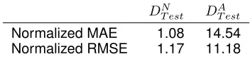
D_{T est}N D_{T est}A

Normalized MAE 1.08 14.54

Normalized RMSE 1.17 11.18

Table 1: Quantitative Analysis: average over all nodes

Node 95-th perc._{N A} 97-th perc._{N A} 99-th perc._{N A}

davide17 0.97 0.89 0.98 0.93 0.99 0.97

davide19 0.97 0.90 0.98 0.94 0.99 0.97

davide45 0.97 0.92 0.98 0.95 0.99 0.98

davide27 0.95 0.90 0.91 0.77 0.86 0.52

davide28 0.94 0.88 0.96 0.89 0.90 0.69

davide29 0.97 0.75 0.98 0.82 0.99 0.85

Average 0.96 0.87 0.96 0.88 0.95 0.82

Table 2: Classification Results

The x-axis andy-axis show, respectively, the time and the normalized reconstruction error (we sum the error for each feature and divide by the number of featuresN F). The re-construction error trend is plotted with a light blue line; the gaps in the line represent periods when the node was idle and that have been removed from the data set.

We observe 6 anomalous periods (highlighted by colored lines along thex-axis): during the first 5 (red lines) the fre-quency governor was set to powersave while during the last one (blue) the governor was set to performance. The restruction error is never exactly zero, but this is not our con-cern: our analysis does not rely on the absolute value of the error, but rather on the relative magnitude of the errors com-puted for different data sets. The reconstruction error is in-deed greater when the nodes are in an anomalous state, as underlined by the higher values in they-axis in the periods corresponding to anomalies. Hence, the autoencoder strug-gles to recreate the “faulty” input data set.

Although the plot shown is promising, it does not actually show that the reconstruction error for unseen healthy input is actually lower than the error committed with anomalous periods. This happens because the normal behaviour data set was randomly split in the subsetDT rainandDT estN and it is

impossible to distinguish between them by simply looking at the plot. However, our insight is backed by the quantitative analysis, as summarized in Table 1. To measure the quality of the anomaly detection we rely on the Mean Absolute Er-ror (MAE) and on the Root Mean Squared ErEr-ror (RSME). For each autoencoder we computed MAE and RSME for every setDT rain,DNT estandD

A T est.

The results obtained for all autoencoders are very simi-lar but in order to make a fair comparison between differ-ent nodes we do not use the absolute values of MAE and RSME but we rather employ a normalized version: the nor-malized MAE (RSME) is obtained by dividing the actual MAE (RSME) by the MAE (RSME) computed forDT rain.

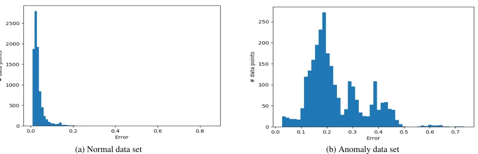
(a) Normal data set (b) Anomaly data set

Figure 2: Error distribution for nodedavide45

between sets. If the normalized error for a test set is close to one this means that the autoencoder was able to reconstruct the input quite well; larger errors imply that the autoencoder was not capable to reproduce the input – these situations are those that we claim to be anomalies.

In Table 1 we can see the results for the test sets. The error for theD_{T est}A is the average value obtained considering both anomaly types. The normalized error forDT rain has not been reported since it is always equal to 1. The values reported in the table are the average computed over all the autoencoders (as many as in the chosen subset of nodes of D.A.V.I.D.E.).

The results clearly indicate that our hypothesis holds true (as hinted also by the previous plot with the reconstruction error). Both the average normalized MAE and RSME for the test set with no anomalies D_{T est}N are very close to 1, suggesting that the autoencoders have correctly learned the correlations between the measured features of a healthy sys-tem. Therefore, when the autoencoders are fed with unseen input that preserve these correlations they can reconstruct it with good precision. On the contrary, the autoencoders cannot correctly reproduce new input that does not resem-ble a healthy system, that is a system in an anomalous state. This is shown by the markedly higher normalized MAE and RSME obtained forD_{T est}A .

Detection Accuracy So far we have observed the recon-struction error trends obtained by our approach based on au-toencoders, but we still have to discuss how the reconstruc-tion error can be used to actually detect an anomaly. Our goal is to identify an error threshold θ to discriminate be-tween normal and anomalous behaviour. In order to do so we shall start by looking at the distributions of the reconstruc-tion errors. Again, we are considering each autoencoder (and thus corresponding node) separately. We distinguish the er-rors distribution for healthy data sets (DT rain∪D_{T est}N ) and for the unhealthy data set (DA_{T est}).

Figure 2 shows the error distributions for the autoencoder corresponding to node davide45– again other nodes have the same behaviour. The graph contains the histograms of the error distributions; in thex-axis we have the

reconstruc-tion error and in the y-axis there is the number of data points with the corresponding error. The left-most sub-figure (Fig. 2a) shows the error distribution for the normal data set (DT rain∪DN

T est) and the other one (Fig. 2b) shows the

dis-tribution for the anomalous data set. It is quite easy to see that the errors distribution of the normal data set is extremely different from the anomalous one.

Since we can clearly distinguish the error distributions we opted for a simple method to classify each data point: if the reconstruction errorEifor data pointiis greater than

a thresholdθ, then the point is “abnormal”; otherwise the data point is considered normal. The next step is to identify the threshold used to classify each data point. We choose as a threshold then-th percentile of the errors distribution of the normal data set, wherenis a value that depends on the specific autoencoder/node. For example in the case of da-vide45(Fig. 2), ifn= 95the threshold is equal to 0.082; this means that 95% of the errors in the normal data set (Fig. 2a) are smaller than this value. Hence, if a data point fed to our trained autoencoder generates an error greater than 0.082 we classify it as anomalous. In order to find the bestnvalue for each autoencoder we employed a simple generate-and-test search strategy, that is we performed experiments with a fi-nite number of values and then chose those guaranteeing the best results in term of classification accuracy.

The table can be divided in three subparts (separated by horizontal lines): 1) the first one contains nodes similar to

davide45, i.e. nodes where most of the anomalies were of type powersave; 2) the second group is comprised of nodes where most of the anomalies had the frequency governor set to performance; 3) the last group (the last row) is the av-erage of the other nodes. In general we can see that the F-score values are very good, highlighting the high accuracy of our approach. A notable difference can be observed between the two sub-groups of nodes. In nodes with a prevalence of powersave anomalies higher thresholds (highern-th values) guarantee better results: this happens because, as seen for instance in Figure 2, the error distributions are more sepa-rable. In the case of nodes characterized by more anomalies of performance type, increasing the threshold does not nec-essarily improve the accuracy – although this can still occur for some nodes. In these nodes it is harder to distinguish nor-mal data points from anonor-malies of type performance (since they behave similarly). Hence, simply increasing the thresh-old is not beneficial, for example for bothdavide27and da-vide28the bestn-th value found through our empirical ex-ploration isn= 94. The underlying reason is that increasing the threshold (for these nodes) leads to a marked increase in the number of false negatives.

Conclusion

In this paper we proposed an approach to detect anoma-lies in a HPC system that reanoma-lies on large data sets collected via a lightweight and scalable monitoring framework and employs autoencoders to distinguish between normal and anomalous system states.

In the future we plan to further validate our method by testing it on a broader set of anomalies. Our goal is to ex-pand the anomaly detection technique in order to be able to also classify different types of anomalies; in addition to rec-ognize that the system is in an anomalous state, the autoen-coder (possibly a refined and more complex version) will be also able to distinguish among different anomaly classes and sources. We also plan to implement our approach in a on-line prototype to perform real-time anomalous detection on a supercomputer, again using D.A.V.I.D.E. as a test bed.

Acknowledgements

This work was partially supported by the European H2020 FET project OPRECOMP (g.a. 732631). We also want to thank CINECA and E4 for granting us the access to their systems.

References

Ahmad, W. A.; Bartolini, A.; Beneventi, F.; Benini, L.; Borghesi, A.; Cicala, M.; Forestieri, P.; Gianfreda, C.; Gregori, D.; and Libri, A. 2017. Design of an energy aware petaflops class high perfor-mance cluster based on power architecture. In2017 IEEE Interna-tional Parallel and Distributed Processing Symposium Workshops (IPDPSW).

Bartolini, A.; Borghesi, A.; Libri, A.; Beneventi, F.; Gregori, D.; Tinti, S.; Gianfreda, C.; and Alto`e, P. 2018. The D.A.V.I.D.E. big-data-powered fine-grain power and performance monitoring sup-port. InProceedings of the 15th ACM International Conference on Computing Frontiers, CF 2018, 303–308.

Baseman, E.; Blanchard, S.; DeBardeleben, N.; Bonnie, A.; and Morrow, A. 2016. Interpretable anomaly detection for monitoring of high performance computing systems. InOutlier Definition, De-tection, and Description on Demand Workshop at ACM SIGKDD. San Francisco (Aug 2016).

Beneventi, F.; Bartolini, A.; Cavazzoni, C.; and Benini, L. 2017. Continuous learning of hpc infrastructure models using big data analytics and in-memory processing tools. InProceedings of the Conference on Design, Automation & Test in Europe. European Design and Automation Association.

Brodowski, D., and Golde, N. 2013. Cpu frequency and voltage scaling code in the linux (tm) kernel.Linux kernel documentation. Cineca inter-university consortium web site. http://www.cineca.it// en. Accessed: 2018-06-29.

Costa, B. S. J.; Angelov, P. P.; and Guedes, L. A. 2015. Fully unsupervised fault detection and identification based on recursive density estimation and self-evolving cloud-based classifier. Neuro-computing150:289–303.

Dani, M. C.; Doreau, H.; and Alt, S. 2017. K-means application for anomaly detection and log classification in hpc. InInternational Conference on Industrial, Engineering and Other Applications of Applied Intelligent Systems, 201–210. Springer.

Dongarra, J. J.; Meuer, H. W.; and Strohmaier, E. 1994. 29th top500 Supercomputer Sites. Technical report, Top500.org. E4 computer engineering. https://www.e4company.com/en/. Feng, W.-c., and Cameron, K. 2007. The green500 list: Encourag-ing sustainable supercomputEncourag-ing.IEEE Computer40(12).

Goodfellow, I.; Bengio, Y.; Courville, A.; and Bengio, Y. 2016.

Deep learning, volume 1. MIT press Cambridge.

Hennessy, J. L., and Patterson, D. A. 2011.Computer architecture: a quantitative approach. Elsevier.

Ince, T.; Kiranyaz, S.; Eren, L.; Askar, M.; and Gabbouj, M. 2016. Real-time motor fault detection by 1-d convolutional neural net-works.IEEE Transactions on Industrial Electronics.

Kingma, D. P., and Ba, J. 2014. Adam: A method for stochastic optimization.arXiv preprint arXiv:1412.6980.

Kiran, B. R.; Thomas, D. M.; and Parakkal, R. 2018. An overview of deep learning based methods for unsupervised and semi-supervised anomaly detection in videos. Journal of Imaging. Kwon, D.; Kim, H.; Kim, J.; Suh, S.; Kim, I.; and Kim, K. 2017. A survey of deep learning-based network anomaly detection.Cluster Computing.

Lee, K. B.; Cheon, S.; and Kim, C. O. 2017. A convolutional neu-ral network for fault classification and diagnosis in semiconductor manufacturing processes. IEEE Transactions on Semiconductor Manufacturing30(2):135–142.

Lv, F.; Wen, C.; Bao, Z.; and Liu, M. 2016. Fault diagnosis based on deep learning. InAmerican Control Conference, 2016. IEEE. Mitchell, T. M. 1999. Machine learning and data mining. Commu-nications of the ACM42(11):30–36.

Ranzato, M. A.; Boureau, Y.-L.; and LeCun, Y. 2008. Sparse fea-ture learning for deep belief networks. InAdvances in neural in-formation processing systems, 1185–1192.

Tuncer, O.; Ates, E.; Zhang, Y.; Turk, A.; Brandt, J.; Leung, V. J.; Egele, M.; and Coskun, A. K. 2017. Diagnosing performance variations in HPC applications using machine learning. In Interna-tional Supercomputing Conference, 355–373. Springer.