Image Formation Using Fast Factorized Backprojection Based on Sub-Aperture and Sub-Image for General Bistatic Forward-Looking SAR with Arbitrary Motion

Image Formation Using Fast Factorized Backprojection

Based on Sub-Aperture and Sub-Image for General Bistatic

Forward-Looking SAR with Arbitrary Motion

Dong Feng1, Daoxiang An1, 2, *, Xiaotao Huang1, 2, and Tian Jin1

Abstract—In this paper, a fast time domain imaging algorithm called bistatic forward-looking fast factorized backprojection algorithm (BF-FFBPA) based on sub-aperture and sub-image is proposed for general bistatic forward-looking synthetic aperture radar (BFSAR) with arbitrary motion. It can not only accurately dispose the large spatial variant range cell migrations and complicated motion errors, but also achieve high imaging efficiency. First, the imaging geometry and signal model are established, and the implementation of back projection algorithm (BPA) in the BFSAR imaging is given to provide a basis for the proposed BF-FFBPA. Then, considering motion errors, the more accurate requirements of splitting sub-aperture and sub-image in the BF-FFBPA is introduced based on the range error analysis to offer the tradeoff between the imaging quality and efficiency. Finally, the implementation and computational burden of the BF-FFBPA is provided and analyzed. Simulated results and evaluations are given to prove the correctness of the theory analysis and the validity of the proposed approach.

1. INTRODUCTION

Synthetic aperture radar (SAR) has gained wide attention these years [1–4], because it can not only get high resolution images of the observed area, but also work day and night under all weather conditions [4]. Therefore, it plays a significant role in both military and civilian fields. However, since the monostatic SAR working in the forward-looking mode has awful azimuth resolution and serious left-right ambiguity problem, its many applications, such as airplane navigation and terminal missile guidance, are greatly limited.

Bistatic SAR refers to SAR systems whose transmitter and receiver are mounted on the separate platforms, which is different from monostatic SAR with collocated transmitter and receiver. Compared to monostatic SAR, bistatic SAR has many advantages, such as obtaining different object scattering information, increasing system survival, and improving stealth in military. More importantly, bistatic SAR can improve azimuth resolution and avoid lift-right ambiguity problem, and thereby can carry out the scene imaging in the forward direction. Different bistatic forward-looking SAR (BFSAR) experiments have been carried out these years [5–8], and a number of challenges have been shown in deploying BFSAR, such as synchronization, coherency and signal processing. The objective of this paper is focused on the signal processing in deploying BFSAR imaging, and imaging algorithm is the key point in the signal processing.

The existing imaging algorithms for BFSAR are divided into two categories: the frequency domain algorithms and the time domain algorithms. The frequency domain algorithms usually aim for minimizing processing time. This aim can lead to a number of limits such as bandwidth, integration

Received 17 January 2017, Accepted 27 March 2017, Scheduled 13 April 2017 * Corresponding author: Daoxiang An ([email protected]).

time, either interpolation or approximation in processing, and memory required by processing which may constrain the usage of the frequency domain algorithms. Recently, some modified frequency domain algorithms are applied on BFSAR imaging, such as the polar format algorithm (PFA) [9, 10], Omega-k algorithm [11], chirp scaling algorithm (CSA) [12], and nonlinear chirp scaling algorithm (NLCSA) [4]. However, the Omega-k algorithm and CSA are only available for the azimuth-invariant BFSAR [3]. Thus, they cannot always satisfy the imaging requirement for the general BFSAR geometry in practice. NLCSA has been used to implement the imaging for azimuth-variant BFSAR [4], but the approximations of handling the spatial-variant range cell migration and range-azimuth coupling may cause large phase errors in particular BFSAR cases.

Compared with the frequency domain algorithms, the back projection algorithm (BPA), which operates in the time domain, can work with almost all configurations of BFSAR in theory. However, the huge computational burden limits the application of the BPA. In order to solve the shortcoming of the BPA, some bistatic fast backprojection algorithms (Bi-FBPA) and bistatic fast factorized backprojection algorithms (Bi-FFBPA) have been proposed in [13–17], and they can be divided into two categories: one works with sub-aperture and polar gird processing [13–16], and the other works on a sub-aperture and sub-image basis [17]. In theory, the extensions of Bi-FBPA and Bi-FFBPA are totally valid for BFSAR without any modification. However, in some special cases of BFSAR, e.g., the centers of the polar grids are very close or even identical to one of the image coordinates, the performance of the Bi-FBPA and Bi-FFBPA which work with sub-aperture and polar grid processing may be very poor since there are difficulties in defining the polar grids [15]. But these difficulties are minimized in Bi-FBPA and Bi-FFBPA which work on a sub-aperture and sub-image basis. Besides, in the intermediate processing step, the Bi-FBPA and Bi-FFBPA which work with sub-aperture and polar gird processing use the polar grids, i.e., working with matrices, while the Bi-FBPA and Bi-FFBPA which work on a sub-aperture and sub-image basis use beams, i.e., working with vectors, hence, the computational burden required by the former may be heavier than the latter. Paper [17] presents the Bi-FBPA and Bi-FFBPA which work on a aperture and image basis, and the requirements of splitting aperture and sub-image are given, but the sampling requirement of the beams was not given, and the requirements of splitting sub-aperture and sub-image are derived only for the linear track bistatic case. However, for the practical BFSAR acquisitions, the radar’s motion errors in the requirements of splitting sub-aperture and sub-image and the sampling requirement of the beams are essential details in the implementation of a precise BF-FFBPA.

Based on the previous work, this paper explores a BF-FFBPA based on sub-aperture and sub-image including the motion errors for the general BFSAR imaging. Firstly, the imaging geometry and signal model are established, and the implementation of BPA in the BFSAR imaging is given. Secondly, based on the range error analysis, the more accurate requirements of splitting sub-aperture and sub-image including motion errors are deduced, which offers the tradeoff between the imaging quality and efficiency. Thirdly, the method of beam forming is proposed, and the sampling requirement of the beams in the beam forming stage of implementation of BF-FFBPA is derived. Finally, the speed-up factor of the proposed BF-FFBPA with respect to BPA is derived.

The remainder of this paper is arranged as follows. Section 2 presents the BPA for general BFSAR with arbitrary motion based on the analysis of the imaging geometry and signal model. Section 3 gives details of the proposed BF-FFBPA. First, more accurate requirements of splitting aperture and sub-image including motion errors are derived. Then, the implementation of the proposed BF-FFBPA is presented. Last but not the least, the computational burden is analyzed. Section 4 shows the simulated results and evaluations to prove the validity of the proposed approach, and Section 5 concludes this paper.

2. BPA FOR GENERAL BFSAR WITH ARBITRARY MOTION

2.1. Imaging Geometry and Signal Model

after the echo signal is received. Thus, the signal can be modeled as a function of two independent variables: fast time and slow time.

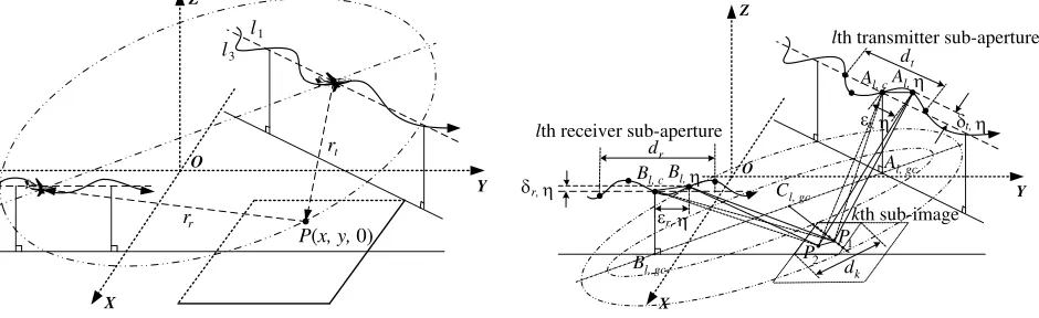
The imaging geometry of general BFSAR with arbitrary motion is shown in Fig. 1. The dashed straight lines l1 and l2 indicate the nominal flight tracks of the transmitter and receiver, while their

actual flight tracks are solid curvesl3 andl4, respectively. The transmitter operates on the side-looking

mode, while the receiver operates on the forward-looking mode. The positions of the transmitter and receiver at the slow time η are denoted as (xt(η), yt(η), zt(η)) and (xr(η), yr(η), zr(η)), respectively.

P(x, y,0) is assumed to be an arbitrary target in the imaging scene. The transmitter and receiver are assumed to be perfectly synchronized. The travelling distance of a radar pulse radiated from a transmitter aperture impinging on this target and then reflected to a receiver aperture position at slow timeη is calculated by

r(η;x, y) = rt(η;x, y) +rr(η;x, y) =

(xt(η)−x)2+ (yt(η)−y)2+ (zt(η))2

+(xr(η)−x)2+ (yr(η)−y)2+ (zr(η))2 (1)

If the transmitted signal is the linear frequency modulation (LFM) pulse signal, and its mathematic expression isp(τ) =wr(τ) exp(j2πfcτ +jπKτ2), whereτ is the fast time,wr(·) the envelope of range,

fc the center frequency, andK the chirp rate, then, the received signal is

s(τ, η) =σPw[τ−r(η;x, y)/c]wa(η−ηc) exp

−j2πfcr(η;x, y)/c+jπK(τ −r(η;x, y)/c)2

(2) whereσP is the reflectivity of the targetP, cthe speed of light, wa(·) the envelope of azimuth, andηc

the synthetic aperture center time. Assume that the time bandwidth product (TBP) of the transmitted LFM pulse signal is very large and that the range envelope wr(·) is a rectangle function. Then, the

received signal after range compression can be approximated as

src(τ, η)σPsinc [B(τ −r(η;x, y)/c)]wa(η−ηc) exp [−j2πfcr(η;x, y)/c] (3)

whereB is the signal bandwidth, and the sinc(·) function is defined as

sinc(x) = sin(πx)/(πx) (4)

Due to the characteristic of azimuth space variance and serious range-azimuth coupling in the BFSAR imaging, it is quite difficult to reconstruct the imaging scene using the frequency domain algorithms. Different from the frequency domain algorithms, the time domain BPA is considered as a linear transformation from the echo signal into the reconstructed image, so it avoids the disposal of the spectrum of the BFSAR target and can be applied directly to the BFSAR imaging with perfect focusing performance.

2.2. BPA for General BFSAR with Arbitrary Motion

For the imaging geometry of general BFSAR with arbitrary motion shown in Fig. 1, assume that (xp, yq)

is an arbitrary point in the discrete imaging scene grid. At slow time η, the travelling distance of a radar pulse radiated from a transmitter aperture impinging on the position (xp, yq) and then reflected

to a receiver aperture position is calculated by Rpq(η) =

(xt(η)−xp)2+ (yt(η)−yq)2+ (zt(η))2+

(xr(η)−xp)2+ (yr(η)−yq)2+ (zr(η))2 (5)

The position (xp, yq) is reconstructed by the superposition of backprojected radar echoes along the

full synthetic aperture, and it is mathematically represented by the integral

h(xp, yq) =

ηc+T /2

η_c−T /2

src(Rpq(η)/c, η) exp [j2πfcRpq(η)/c]dη (6)

where T is the synthetic aperture time. An ellipsoidal mapping is the basic for the backprojection in BFSAR. The foci of the ellipsoid are defined by the actual aperture positions of the transmitter and receiver platforms, as shown in Fig. 1.

3. BF-FFBPA FOR GENERAL BFSAR WITH ARBITRARY MOTION

To reduce the computational burden of the BPA for general BFSAR imaging, a BF-FFBPA based on sub-aperture and sub-image for general BFSAR with arbitrary motion is presented in this section.

The proposed BF-FFBPA processes the BFSAR data on a sub-aperture and sub-image basis, i.e., local processing. This means that the complete transmitter and receiver apertures are split into a number of sub-apertures while the full reconstructed scene is segmented into a number of sub-images. Due to the local processing, the efficiency of image formation is significantly improved, whereas the range errors are caused in the processing stages, and the phase errors appear in the reconstructed image. The lower the number of sub-apertures and sub-images is, the shorter processing time BF-FFBPA requires, whereas the bigger phase error in the reconstructed image appears, so there is a tradeoff between the imaging efficiency and the imaging quality. Therefore, the requirements of splitting sub-aperture and sub-image play a significant role in the BF-FFBPA processing.

X

Y Z

O 2

l

1

l

t

r

r

r

3

l

4

l

P(x, y, 0)

Figure 1. Imaging geometry with arbitrary motion of the general BFSAR.

X

Y Z

O lth receiver sub-aperture

P₂ P1

lth transmitter sub-aperture

kth sub-image

d_k

δr, η

εr, η d_r

l, c B Bl, η

l, gc B

l, gc C

l, gc A

dt

l, c A Al, η

εt, η δt, η

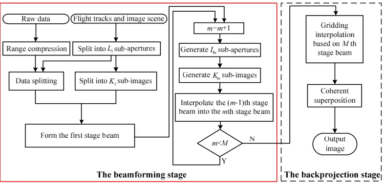
Figure 2. Range error analysis in BF-FFBPA for general BFSAR with arbitrary motion.

3.1. Requirements of Splitting Sub-Aperture and Sub-Image Considering Motion Errors The proposed BF-FFBPA is able to handle nonlinear flight tracks of the transmitter and receiver as the derivation of the requirements of splitting sub-aperture and sub-image considers the motion errors. The motion errors here refer to the trajectory deviation errors.

In order to investigate the requirements of splitting sub-aperture and sub-image, we need to calculate the bistatic range error between the true travel distance of radar pulse and the processed travel distance. In the lth transmitter sub-aperture, the kth sub-image and the corresponding lth receiver sub-aperture, the bistatic range error between the true travel distance of radar pulse and the processed travel distance are depicted in Fig. 2. Al,c and Bl,c are the positions of the lth transmitter

and receiver sub-aperture center, respectively. Let dt,dr and dk denote the length of the transmitter

sub-aperture, the length of the receiver sub-aperture and the maximum dimension of the sub-image, respectively. Al,η andBl,η are the transmitter and receiver aperture positions at slow time η belonging

to thelth sub-aperture, respectively. Let εt,η be the distance between the positionsAl,c and Al,η along

the transmitter nominal track. δt,η is the across-track deviation of Al,η from the transmitter nominal

track. Similarly, we useεr,η to denote the distance between the positionsBl,candBl,η along the receiver

nominal track, and δr,η to denote the across-track deviation of Bl,η from the receiver nominal track.

The length of the beam belonging to thekth sub-image is limited by two dotted-dashed ellipses in the ground. The foci of the ellipses are Al,gc and Bl,gc, which are the projections in the ground plane of

Al,c andBl,c, respectively. Cl,gc is the center of the ellipses. P1 is the position of the ith sample of the

beam belonging to thekth sub-image. P2 is an arbitrary image pixel in thekth sub-image whose value

is mapped by the ith sample of the beam belonging to the kth sub-image.

Bl,η is R = Rt+Rr, where Rt and Rr indicate the lengths of the straight lines Al,ηP2 and Bl,ηP2,

respectively. However, the processed travel distance is R = R_t+R_r, where R_t and R_r indicate the lengths of the straight lines Al,ηP1 and Bl,ηP1, respectively. The difference between the true travel

distance R and the processed travel distance R causes a range error and thus a phase error in the reconstructed BFSAR image.

To calculate the range error in the BF-FFBPA for the general BFSAR with arbitrary motion, some auxiliary variables need to be introduced. Let ρt, σt, ρr, and σr be the lengths of the straight

lines Al,cP1, Al,cP2, Bl,cP1 and Bl,cP2, respectively. Besides, we use βt to denote the angle between

the vector −−−→Al,cP1 and the transmitter nominal motion direction, and Δβt to denote the angle between

the vectors −−−→Al,cP1 and −−−→Al,cP2. Similarly, the angle between the vector −−−−→Bl,cP1 and the receiver nominal

motion direction is denoted by βr, and the angle between the vectors −−−−→Bl,cP1 and −−−−→Bl,cP2 is denoted by

Δβr. Thus, the true travel distanceR and the processed travel distanceR are determined by the law

of cosine as

R=Rt+Rr=

σ_t2+ε_t,η2 −2σtεt,ηcos (βt+Δβt+ϕt)+

σ2

r +εr,η2 −2σrεr,ηcos (βr+ Δβr+ϕr) (7)

R =R_t+R_r=

ρ2

t +ε

₂

t,η −2ρtεt,ηcos (βt+ϕt) +

ρ2

r+εr,η2 −2ρrεr,ηcos (βr+ϕr) (8)

where ε_t,η =

ε2_t,η+δ2_t,η and ε_r,η =

ε2

r,η+δ2r,η indicate the lengths of the straight lines Al,cAl,η

and Bl,cBl,η, respectively. ϕt and ϕr are the angles which are defined by ϕt = arctan(δt,η/εt,η) and

ϕr = arctan(δr,η/εr,η), respectively. Applying the Taylor expansion for the square root terms on the

right hand side of (7) and taking only the first two terms of the Taylor series into account, the true travel distance is then approximated by

R≈σt+σr−εt,ηcos (βt+ Δβt+ϕt)−εr,ηcos (βr+ Δβr+ϕr) (9)

Similarly, the processed travel distance can be approximated by

R ≈ρt+ρr−εt,ηcos (βt+ϕt)−εr,ηcos (βr+ϕr) (10)

According to the principle of ellipsoidal mapping,P1 and P2 are in the same ellipse whose foci are

Al,c and Bl,c. Thus, due to the characteristics of an ellipse, the equationσt+σr =ρt+ρr always holds

true. Then, the range error is calculated as follows:

ΔR = (R−R

₎

2 cos(α) =

ε_t,η[cos (βt+ϕt)−cos (βt+ Δβt+ϕt)]

2 cos(α) +

ε_r,η[cos (βr+ϕr)−cos (βr+ Δβr+ϕr)]

2 cos(α)

=

ε2_t,η +δ_t,η2 sin

βt+ϕt+

Δβt 2 sin Δβt 2 cos(α) + ε2

r,η+δr,η2 sin

βr+ϕr+

Δβr 2 sin Δβr 2 cos(α) (11)

whereα is half of the angle between the vectors−−−−→P2Al,η and −−−−→P2Bl,η. Assume that the maximum

across-track deviations of transmitter and receiver from the nominal across-track along the full synthetic aperture areδt,max andδr,max, respectively. Then, the following inequations hold true:

⎧ ⎪ ⎪ ⎪ ⎪ ⎪ ⎪ ⎨ ⎪ ⎪ ⎪ ⎪ ⎪ ⎪ ⎩

0≤εt,η ≤dt/2

0≤εr,η ≤dr/2

0≤δt,η ≤δt,max

0≤δr,η ≤δr,max

sin (βt+ϕt+ Δβt/2)≤1

sin (βr+ϕr+ Δβr/2)≤1

(12)

Let εk, r1 and r2 be the lengths of the straight lines P1P2,Al,cP2 and Bl,cP2, respectively. Then

we can see from Fig. 2 that _⎧

⎪ ⎪ ⎨ ⎪ ⎪ ⎩ sin Δβt 2 ≈ ε_k

2r₁ ≤ d_k

4r_1,min

sin

Δβr

2

≈ ε_k

2r2 ≤ d_k

4r_2,min

wherer1,minandr2,minare the minimum values ofr1andr2along the full synthetic aperture, respectively.

Combining Eqs. (11), (12) and (13), the upper bound of the range error can be represented as

ΔR≤ dk

(dt/2)2+δ2t,max

4r1,mincos(α)

+ dk

(dr/2)2+δr,2max

4r2,mincos(α)

(14)

Assume that the lengths of the full transmitter aperture and receiver aperture are St and Sr and

that the size of imaging scene is Ix×Iy. Then the number of sub-apertures isL=St/dt=Sr/dr, and

the number of sub-images is K = 2IxIy/d2k. Therefore, the phase error appears in the reconstructed

image caused by the range error can be represented as

Δφ= 2π λΔR≤

π2IxIy/K

4λmincos(α) ⎡ ⎣

(St/L)2+ 4δ2t,max

r1,min

+

(Sr/L)2+ 4δ2r,max

r2,min

⎤

⎦ (15)

whereλmin=c/(fc+B/2) denotes the minimum wavelength of the signal. As shown in [3] and [17], if

the maximum phase error is not bigger thanπ/8, the effect caused by the phase error can be neglected in the far-field SAR imaging. Thus, the splitting requirements of sub-aperture and sub-image can be represented as

K ≥ 8IxIy

(St/L)2+ 4δt,2max/r1,min+

(Sr/L)2+ 4δr,2max/r2,min 2

λ2

mincos2(α)

(16)

Equation (16) indicates that if the number of sub-aperturesLis selected, the number of sub-images K should be selected no less than the right-hand side of Eq. (16).

3.2. Sampling Requirement of the Beams and Implementation

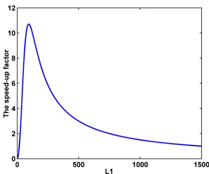
Reconstructing the BFSAR image by the proposed BF-FFBPA is divided into two stages, i.e., the beamforming stage and the backprojection stage. The method of beamforming in the first beamforming stage of the proposed BF-FFBPA is that all radar echoes after demodulation and range compression belonging to a sub-aperture are backprojected into the range center line in the ground plane belonging to a sub-image to form one beam. Take thelth sub-apertures and thekth sub-image shown in Fig. 2 for example, the range center line belonging to thekth sub-image is defined by the straight line crossing through the center of this sub-image and the center of the ellipse whose foci are the projections of the centers of the lth transmitter and receiver sub-apertures. In practice, the range center line is sampled to generate some discrete positions, and the beam is formed by backprojecting the radar echoes to these positions. The minimum length of the beam is limited by two dotted-dashed ellipses in the ground shown in Fig. 2.

In order to avoid aliasing in the beamforming, the sampling of the beam must satisfy requirement. Assume that the positions of the first and the last samples of the beam belonging to the lth sub-apertures, and thekth sub-image is denoted byPfirst andPlast, respectively. LetNb, Δb, and Δr be the

number of samples that the beam consists of, the ground sampling interval of the beam, and the range sampling interval of the signal, respectively. Assume that the travel distances of a radar pulse radiated from the center of thelth transmitter sub-aperture impinging on the positionsPfirstand Plast, and then

reflected to the corresponding center of the lth receiver sub-aperture areRfirst and Rend, respectively.

LetD be the length of the straight linePfirstPlast. Thus, the following equations hold true:

D=NbΔb

Rend−Rfirst =NbΔr

(17)

According to the Nyquist sampling theorem, the range sampling interval of the signal Δr must satisfy the requirement Δr≤c/B, then the ground sampling interval of the beam Δbshould satisfy the following requirement:

Δb≤ cD

B(Rend−Rfirst)

m L

m K 1

L

1 K

Figure 3. The flowchart of the implementation of the proposed BF-FFBPA.

Please note that the BF-FFBPA performs multiple beamforming stages before the backprojection stage. Fig. 3 shows the flowchart of the implementation of the proposed algorithm. The processing in the red solid rectangle is the beamforming stage, and the processing in the black dashed rectangle is the backprojection stage.

In the first beamforming stage, the full transmitter and receiver apertures are firstly split intoL1

sub-apertures which require a similar split of the range-compressed data at the same time, while the full reconstructed scene is segmented intoK1 sub-images according to Eq. (16). Take thel1th (1≤l1≤L1)

sub-apertures and the k1th (1 ≤ k1 ≤ K1) sub-image for example. Assume that (xl1,k1, yl1,k1) is the

position of an arbitrary sample of the beam belonging to thel1th sub-apertures and thek1th sub-image,

then the value of this sample is determined by

bl1,k1(xl1,k1, yl1,k1) =

η_l1+T_s/2

η_l1−Ts/2

src(Rl1,k1(η)/c, η) exp [j2πfcRl1,k1(η)/c]dη (19)

where ηl1 is the time instant corresponding to the l1th centers of the sub-apertures, and Ts is the

integration time of thel1th sub-apertures. Rl1,k1(η) is calculated by

Rl₁,k₁(η) =

(xl1

t (η)−xl₁,k₁)2+ (ylt1(η)−yl₁,k₁)2+ (ztl1(η))2

+

(xlr1(η)−xl₁,k₁)2+ (yrl1(η)−yl₁,k₁)2+ (zlr1(η))2 (20)

where (xl_t1(η), y_tl1(η), zl_t1(η)) and (xl1

r(η), ylr1(η), zrl1(η)) denote the transmitter and receiver aperture

positions belonging to the l1th sub-apertures, respectively. Please note that yl1,k1 is the function of

xl1,k1 in the range center line, i.e., yl1,k1 = f(xl1,k1). Thus, bl1,k1(xl1,k1, yl1,k1) can be represented

as bl1,k1(xl1,k1, yl1,k1) = bl1,k1(xl1,k1, f(xl1,k1)) = bl1,k1(xl1,k1). Assume that the travel distance

of a radar pulse radiated from the center of the l1th transmitter sub-aperture impinging on the

position (xl,k, yl,k) and then reflected to the center of the l1th receiver sub-aperture is denoted by

R_ll1₁,c_,k1(xl1,k1, yl1,k1), which is calculated by

Rl_l1,c

1,k₁(xl1,k1, yl1,k1) =

(xl_t1,c−xl1,k1)2+ (y l1,c

t −yl1,k1)2+ (z l1,c t )2

+

(xlr1,c−xl1,k1)2+ (y l₁,c

r −yl1,k1)2+ (z l₁,c

r )2 (21)

where (x_tl1,c, y_tl1,c, zl_t1,c) and (xrl1,c, ylr1,c, zlr1,c) are the positions of the centers of the l1th transmitter

and receiver sub-apertures, respectively. Similarly, R_ll1,c

R_ll1,c

1,k₁(xl1,k1, yl1,k1) = R l1,c

l₁,k₁(xl1,k1). Therefore, xl1,k1 is the inverse function of R l1,c

l₁,k₁, i.e., xl1,k1 =

g(Rl_l1,c

1,k₁). Therefore, the beam formed in thel1th sub-apertures andk1th sub-image can be represented

as

bl₁,k₁(xl₁,k₁, yl₁,k₁) =bl₁,k₁

R_ll1,c

1,k1

(22) In themth (2≤m ≤M, and M is the processing stages of beamforming) beamforming stage, the number of sub-apertures is combined intoLm, and the number of sub-images is changed into Km. The

new sets of beams in the mth stage are generated from the old sets of beams formed in the (m−1)th beamforming stage. Assume that (xl_m,k_m, yl_m,k_m) is the position of an arbitrary sample of the beam

belonging to thelmth (1≤lm ≤Lm) sub-apertures and the kmth (1≤km ≤Km) sub-image in themth

beamforming stage, andγ sub-apertures are combined into one sub-aperture each time, then the value of this sample is determined by

blm,km(xlm,km, ylm,km) =blm,,km

Rl_lm,c

m,km

=

lmγ

lm−1=1+(lm−1)γ

blm−1,,km−1

Rl_lm−1,c

m,km

(23)

where

Rl_lm_m,c_,km =

xl_tm,c−xlm,km 2

+

y_tlm,c−ylm,km 2

+

z_tlm,c

2

+

xlrm,c−xlm,km 2

+

yrlm,c−ylm,km 2

+

zrlm,c

2

(24) and

Rl_lm_m−_,k1_m,c =

xl_tm−1,c−xlm,km 2

+

yl_tm−1,c−ylm,km 2

+

z_tlm−1,c

2

+

xlrm−1,c−xlm,km 2

+

yrlm−1,c−ylm,km 2

+

zrlm−1,c

2

(25)

In Eq. (25), the coordinates (xl_tm,c, y_tlm,c, z_tlm,c) and (xlrm,c, yrlm,c, zlrm,c) indicate the centers of the

lmth transmitter and receiver sub-apertures in the mth beamforming stage, respectively. In Eq. (26),

the coordinates (x_tlm−1,c, y_tlm−1,c, z_tlm−1,c) and (xrlm−1,c, ylrm−1,c, zrlm−1,c) indicate the centers of the lm−1th

transmitter and receiver sub-apertures in the (m−1)th beamforming stage, respectively.

In the backprojection stage, the beams formed in theMth beamforming stage are backprojected into the imaging grid to reconstruct the final BFSAR image. The number of sub-apertures is LM and

the number of sub-images is KM now. Take an arbitrary point in the kMth (1≤kM ≤KM) sub-image

grid for example. (xp,kM, yq,kM) is supposed to be the position of this point, then the value of this point

after backprojecting is calculated by

hk_M (xp,k_M, yq,k_M) = L_M

l_M=1

bl_M,k_M

R_p,q,klM,c

M

(26)

where

Rl_p,q,kM,c

M =

xl_tM,c−xp,k_M

2

+

y_tlM,c−yq,k_M

2

+

z_tlM,c

2

+

xlrM,c−xp,k_M

2

+

yrlM,c−yq,k_M

2

+

zlrM,c

2

(27)

The coordinates (x_tlM,c, yl_tM,c, z_tlM,c) and (xrlM,c, yrlM,c, zrlM,c) indicate the centers of thelMth transmitter

and receiver sub-apertures, respectively. Therefore, the sampled version of thekMth sub-image can be

represented in the matrix form as follows:

HkM = ⎡ ⎢ ⎣

hk_M(x1,k_M, y1,k_M) hk_M (x1,k_M, y2,k_M) . . .

hk_M(x2,k_M, y1,k_M) . .. ...

..

. . . . . ..

⎤ ⎥

The full BFSAR image is finally reconstructed by a union of all sub-images in a correct order.

3.3. Computational Burden

It is seen from the implementation of the proposed BF-FFBPA that the computational burden is mostly contributed by three parts, i.e., backprojecting the radar echoes into the range center lines, interpolating the old beams into the new beams, and interpolating the final beams into the image grids.

Assume that the number of transmitter and receiver aperture positions is Nl, and the imaging

scene grid has the dimensionsNx×Ny. In the first beamforming stage, the number of samples included

in one beam is assumed to be Nb, then the computational burden of backprojecting the radar echoes

into the range center lines C1 is proportional to L1K1×(Nl/L1)×Nb, i.e., C1 ∝ K1NlNb. In the

mth beamforming stage, the new beams are interpolated from the old beams formed in the (m−1)th beamforming stage, so the computational burden of interpolating the (m−1)th beams into the mth beams is proportional toγNbL1K1. Thus afterM stages processing of beamforming, the computational

burden C2 can be represented asC2 ∝M γNbL1K1. In the backprojection stage, the beams formed in

the Mth beamforming stage are backprojected to the imaging scene grid, i.e., interpolating the final beams into the image grids. The needed number of operations can be represented asC3 ∝L1NxNy/γM.

Therefore, the total computational burden of the proposed BF-FFBPA is

CBF-FFBPA=C1+C2+C3 ∝K1NlNb+M γNbL1K1+L1NxNy/γM (29)

Analogously, the computational burden of the BPA is given by

CBPA∝NlNxNy (30)

The speed-up factor of the proposed BF-FFBPA with respect to the BPA can be represented as

κBF-FFBPA =

CBPA

CBF-FFBPA ∝

NlNxNy

K1NlNb+M γNbL1K1+L1NxNy/γM

(31)

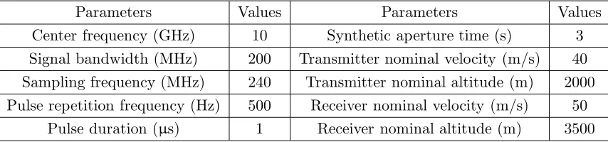
Equation (16) shows that K1 can be represented as the function of L1, thus the speed-up factor

κBF-FFBPA is proportional to the function ofL1. Based on Eqs. (16) and (31), the variation trend of the

speed-up factorκBF-FFBPA with respect toL1 is shown in Fig. 4. It is seen from Fig. 4 that the value of

the speed-up factor κBF-FFBPA changes along with the variety of the number of the sub-apertures L1,

and the maximum speed-up factor can be obtained whenL1lies on some location. That is to say, there

is an optimal splitting of sub-aperture to make the imaging efficiency to be improved highest compared with the BPA.

Figure 4. The variation trend of the speed-up factor with respect toL1.

4. SIMULATION RESULTS AND EVALUATIONS

In order to prove the validity of the proposed BF-FFBPA, a comparative simulation experiment for the general BFSAR imaging is carried out in this section. The image reconstructed using BPA is used as a reference for comparison, since BPA can be seen as the most accurate imaging algorithm without any errors.

4.1. Arrangement

The simulation parameters are shown in Table 1, and the imaging geometry in this simulation is shown in Fig. 5. The transmitter works on the side-looking mode, and the angle between the nominal track of transmitter andY-axis is 15◦. The receiver works on the forward-looking mode, and the nominal track of receiver is parallel to Y-axis. The transmitter is assumed to be synchronized with the receiver perfectly. The same motion errors are added to the nominal flight tracks of the transmitter and receiver. The error added in X-axis is δx = 2 sin(2π(0.3/3)η) + 0.1η, the errors added in Y-axis is

δy = 3 sin(2π(0.8/3)η) + 0.2η, and δz = 5 sin(2π(0.5/3)η) + 0.3η is the errors added in Z-axis.

Table 1. Simulation parameters.

Parameters Values Parameters Values

Center frequency (GHz) 10 Synthetic aperture time (s) 3 Signal bandwidth (MHz) 200 Transmitter nominal velocity (m/s) 40 Sampling frequency (MHz) 240 Transmitter nominal altitude (m) 2000 Pulse repetition frequency (Hz) 500 Receiver nominal velocity (m/s) 50

Pulse duration (µs) 1 Receiver nominal altitude (m) 3500

The simulated ground scene consists of nine stationary point-like targets labeled as A-I in turn, which are equally spaced in an area of 300 m×300 m (X×Y). The intervals of the targets inX and Y-directions are both 100 m, and the scene center position is (2000, 0, 0) m. The radar cross sections (RCS) of these targets are normalized to be 1 m2.

4.2. Imaging Results

To examine the proposed algorithm, we use the BPA and the proposed BF-FFBPA to reconstruct the same scene with the same simulated BFSAR data, and a comparative study between the results focused by the BPA and the proposed BF-FFBPA is used to prove the validity of the proposed algorithm.

The BPA can be implemented conveniently, but the implementation of the proposed BF-FFBPA needs to select the parameters carefully. The parameters here refer to the number of sub-apertures, number of sub-images and number of samples included in one beam in the beamforming stage, and the selections of these parameters for the BF-BBFPA directly affect the imaging efficiency and quality.

From Fig. 4 we can know that there is an optimal splitting of sub-aperture which can make the speed-up factor arrive at maximum, and the optimal sub-aperture size in this simulation is calculated to beL1= 93. Thus, the number of sub-images can be selected to beK1= 1521 according to Eq. (16).

In order to avoid aliasing in the beamforming, the number of samples included in one beam is selected to beNb = 128.

(a) (b) (c)

Figure 6. Focused results by different algorithms. (a) Distribution of targets. (b) BPA. (c) The proposed BF-FFBPA.

(a) (b) (c) (d)

Figure 7. Target A. (a) Focused by BPA. (b) Focused by BF-FFBPA. (c) Cuts in X direction. (d) Cuts inY direction.

(a) (b) (c) (d)

Figure 8. Target E. (a) Focused by BPA. (b) Focused by BF-FFBPA. (c) Cuts in X direction. (d) Cuts inY direction.

4.3. Evaluation

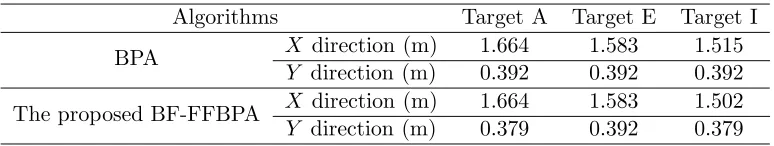
To further evaluate the performance of the proposed algorithm, three focused point-like targets labeled as A, E and I are extracted from Fig. 6. The contours of targets A, E and I in the range [−30, 0] dB are shown in Figs. 7, 8 and 9. Besides, the cuts containing the peak mainlobe in theX and Y directions of the considered point-like targets are also shown to compare the algorithms’ performance. As observed from Figs. 7∼9, the contours and cuts of the considered targets focused by the BPA and the proposed BF-FFBPA are very similar.

(a) (b) (c) (d)

Figure 9. Target I. (a) Focused by BPA. (b) Focused by BF-FFBPA. (c) Cuts in X direction. (d) Cuts inY direction.

Table 2. Measured HPBWs of the extracted targets.

Algorithms Target A Target E Target I BPA X direction (m) 1.664 1.583 1.515

Y direction (m) 0.392 0.392 0.392 The proposed BF-FFBPA X direction (m) 1.664 1.583 1.502 Y direction (m) 0.379 0.392 0.379

approximations in BF-FFBPA.

To prove the imaging efficiency of the proposed algorithm, the processing time of the proposed BF-FFBPA and BPA is measured in the Matlab R2013b on a computer with a 3.20 GHz Intel processor and 8.00 GB Random Access Memory (RAM). The average processing time of the BPA and the proposed BF-FFBPA are 1323 s and 138 s, respectively. Compared with BPA, the speed-up factor of the proposed BF-FFBPA is about 9.6. Therefore, a hint of the processing time reduction is clearly given by the measured results.

5. CONCLUSION

This paper presents a BF-FFBPA based on sub-aperture and sub-image for general BFSAR considering motion errors. It can not only accurately dispose the large spatial variant range cell migrations and complicated motion error, but also achieve high imaging efficiency. The imaging geometry and signal model are firstly established, based on which the difficulty of using frequency domain algorithm to reconstruct the BFSAR image is analyzed, and the implementation of BPA to reconstruct the BFSAR image is given. To reduce the computational burden, the BF-FFBPA based on aperture and sub-image is successively proposed. The requirement of splitting sub-aperture and sub-sub-image is deduced considering motion errors in the general BFSAR configuration, and the sampling requirement of the beams in the beamforming stages of the BF-FFBPA is given. Besides, the implementation of the proposed algorithm is presented, and the computational burden is discussed. Finally, the correctness of the theory analysis and validity of the proposed approach are proved by the simulations and evaluations.

ACKNOWLEDGMENT

This work was supported by the National Natural Science Foundation of China under Grants 61571447 and 61372161.

REFERENCES

2. An, D. X., Y. H. Li, X. T. Huang, X. Y. Li, and Z. M. Zhou, “Performance evaluation of frequency-domain algorithms for chirped low frequency UWB SAR data processing,” IEEE J. Sel. Topics Appl. Earth Observ., Vol. 7, No. 2, 678–690, 2014.

3. Xie, X. T., D. X. An, X. T. Huang, and Z. M. Zhou, “Fast time-domain imaging in elliptical polar coordinate for general bistatic VHF/UHF ultra-wideband SAR with arbitrary motion,” IEEE J. Sel. Topics Appl. Earth Observ., Vol. 8, No. 2, 879–895, 2014.

4. Chen, S., Y. Yuan, S. N. Zhang, H. C. Zhao, and Y. Chen, “A new imaging algorithm for forward-looking missile-borne bistatic SAR,” IEEE J. Sel. Topics Appl. Earth Observ., Vol. 9, No. 4, 1543–1552, 2016.

5. Yang, J. Y., Y. L. Huang, H. G. Yang, J. J. Wu, W. C. Li, Z. Y. Li, and X. B. Yang, “A first experiment of airborne bistatic forward-looking SAR preliminary results,” Proc IEEE Int. Geosci. Remote Sens. Symp. (IGARSS), 4202–4204, Melbourne, VIC, Australia, 2013.

6. Espeter, T., I. Walterscheid, J. Klare, A. R. Brenner, and J. H. G. Ender, “Bistatic forward-looking SAR: Results of a spaceborne-airborne experiment,” IEEE Geosci. Remote Sens. Lett., Vol. 8, No. 4, 765–768, 2011.

7. Wu, J. J., Y. L. Huang, J. Y. Yang, W. C. Li, and H. G. Yang, “First results of bistatic forward-looking SAR with stationary transmitter,”Proc IEEE Int. Geosci. Remote Sens. Symp. (IGARSS), 1223–1226, Vancouver, BC, Canada, 2011.

8. Walterscheid, I., A. R. Brenner, and J. Klare, “Radar imaging with very low grazing angles in a bistatic forward-looking configuration,” Proc IEEE Int. Geosci. Remote Sens. Symp. (IGARSS), 327–330, Munich, Germany, 2012.

9. Zhang, H. R., Y. Wang, and J. W. Li, “New applications of parameter-adjusting polar format algorithm in spotlight forward-looking bistatic SAR processing,” Proc. Asian Pacific Synth. Aperture Radar (APSAR), 384–387, Tsukuba, Japan, 2013.

10. Sun, J. P., Y. Lv, W. Hong, and S. Y. Mao, “The polar format imaging algorithm for forward-looking bistatic SAR,” Proc. Eur. Conf. Synth. Aperture Radar (EUSAR), 1–4, Friedrichshafen, Germany, 2008.

11. Shin, H. S. and J. T. Lim, “Omega-k algorithm for airborne forward-looking bistatic spotlight SAR imaging,”IEEE Geosci. Remote Sens. Lett., Vol. 6, No. 2, 312–316, 2009.

12. Wu, J. J., J. Y. Yang, Y. L. Huang, and H. G. Yang, “Focusing bistatic forward-looking SAR using chirp scaling algorithm,”Proc. IEEE Radar Conf. (RADAR), 1036–1039, Kansas, MO, USA, 2011. 13. Rodriguez-Cassola, M., P. Prats, G. Krieger, and A. Moreira, “Efficient time-domain image formation with precise topography accommodation for general bistatic SAR configurations,”IEEE Trans. Aerosp. Electron. Syst., Vol. 47, No. 4, 2949–2966, 2011.

14. Vu, V. T. and M. I. Pettersson, “Fast backprojection algorithms based on subapertures and local polar coordinates for general bistatic airborne SAR systems,”IEEE Trans. Geosci. Remote Sens., Vol. 54, No. 5, 2706–2712, 2016.

15. Vu, V. T., T. K. Sj¨ogren, and M. I. Pettersson, “SAR imaging in ground plane using fast backprojection for mono- and bistatic cases,” Proc. IEEE Radar Conf. (RADAR), 0184–0189, Atlanta, GA, USA, 2012.

16. Shao, Y. F., R. Wang, Y. K. Deng, Y. Liu, R. P. Chen, G. Liu, and O. Loffeld, “Fast backprojection algorithm for bistatic SAR imaging,”IEEE Geosci. Remote Sens. Lett., Vol. 10, No. 5, 1080–1084, 2013.