Combining difference and equivalence test results in spatial maps

R E S E A R C H

Open Access

Combining difference and equivalence test

results in spatial maps

Thomas Waldhoer

1

, Harald Heinzl

2*

Abstract

Background:Regionally partitioned health indicator values are commonly presented in choropleth maps. Policymakers and health authorities use them among others for health reporting, demand planning and quality assessment. Quite often there are concerns whether the health situation in certain areas can be considered different or equivalent to a reference value.

Results:Highlighting statistically significant areas enables the statement that these areas differ from the reference value. However, this approach does not allow conclusions which areas are sufficiently close to the reference value, although these are crucial for health policy making as well. In order to overcome this weakness a combined integration of statistical difference and equivalence tests into choropleth maps is suggested and the approach is exemplified with health data of Austrian newborns.

Conclusions:The suggested method will improve the interpretability of choropleth maps for policymakers and health authorities.

Background

A choropleth map consists of coloured or patterned areas which represent different values or categories of a quantitative attribute. Displaying health information data in choropleth maps has become common practice in spatial epidemiology.

Statistically significant deviations of the depicted values from a reference value are often highlighted in such maps. Their results, however, may lead to unwanted concerns and bewilderment in certain signifi-cantly worse regions. Inhabitants of those regions may put political pressure on local authorities and govern-mental agencies. However, in spatial units with many observed events, even tiny and irrelevant effects may show statistical significance. On the other hand, statisti-cal difference tests usually have little statististatisti-cal power for areas exhibiting few events which could intuitively lead to the false impression that areas with non-signifi-cant test results are close to the reference value.

Equivalence tests can provide useful information in addition to difference tests as the former require the

specification of a conclusively substantiated equivalence range. We suggest the combined use of both difference and equivalence tests in spatial maps. We exemplify that this combined approach provides more insight into spa-tial conditions than sole difference tests. We think that it can considerably enhance the illustrative capability of choropleth maps in public health and epidemiology.

The paper is organised as follows. Basic ideas, statisti-cal methods, and the combined approach are presented before the combined approach is applied to two data sets. A discussion and conclusions section closes the paper.

Methods

The main features of difference and equivalence tests are motivated with the one-sample t-test. Based on it, the combination of both test principles is thoroughly ventilated. Although these considerations are general by nature, the application of permutation tests may pose additional questions which are considered and exempli-fied with standard mortality ratios (SMR’s). Multiple testing and a Bayesian alternative approach are briefly considered as well.

* Correspondence: [email protected]

2

Center for Medical Statistics, Informatics, and Intelligent Systems, Medical University of Vienna, Spitalgasse 23, A-1090 Vienna, Austria

Full list of author information is available at the end of the article

The one-sample t-test as difference test

Consider a single group with normally distributed out-comes, X ~ N(μ,s2), whereμ ands2 are the unknown population mean and variance. The research question whether the population meandiffersfrom a chosen con-stantc is usually answered with a one-sample t-test of the null hypothesis H0: μ=con a prespecified

signifi-cance level a. The corresponding non-directional two-sided alternative hypothesis is denoted by HA:μ≠c.

The null hypothesis H0: μ =c can be considered as

intersection of two one-sided null hypotheses H01:μ≤c

and H02:μ≥c, respectively. Testing them can be

under-stood as a closed testing procedure which holds the multiple levelaand a confirmatory directional conclu-sion is possible (see e.g. [1], [2]). The corresponding one-sided directional alternatives are HA1:μ>cand HA2:

μ<c, respectively.

In the case of one-sample t-test the application of a two-sided level a test comprises the computation of a realisationtof a test statistic T, and its comparison with some lower and upper critical valuescritlowand critupp, respectively. If t ∉ [critlow,critupp], then H0 will be

rejected for the non-directional hypothesis testing approach; ift>critupp ort<critlow, then H01 or H02will

be rejected for the directional approach, respectively. The use of a two-sided (1 - a) -confidence interval provides an alternative way to perform a two-sided level a difference test. Let ⎡⎣xlow, /2,xupp,1−/2⎤⎦ denote the common symmetric (1 -a) -confidence interval forμ. If

c∉ ⎡⎣x_low,2,x_upp,1−2⎤⎦, then H0 will be rejected for

the non-directional hypothesis testing approach. If x_low,2>c or x_upp,1−2<c, then H01 or H02 will be

rejected for the directional approach, respectively. Three crucial confidence interval scenarios as results of a dif-ference test are depicted in Figure 1. Note that, even if not intended, confidence intervals always provide direc-tional information as well.

The one-sample t-test as equivalence test

A not significantdifferencetest cannot be interpreted as acceptance of the null hypothesis. The population mean μis only consideredequivalentto a chosen constantcif they do not differ too much, that is, ifμ Î(c- Δ1, c+

Δ2). The acceptable differences Δ1and Δ2 re called

equivalence margins and have to be predetermined. Often, Δ1=Δ2 will be chosen for a normally distributed

outcome. The equivalence limitsc -Δ1 and c+Δ2form

the equivalence range.

Statistical equivalence testing is commonly based on a two one-sided tests (TOST) approach. If both one-sided

null hypotheses _Η01∗ : _{≤ −}c _Δ1and _Η02∗ : _{≥ +}c _Δ2

are rejected at a significance level a each, then the population meanμcan be declaredequivalenttoc.

The TOST approach can be easily performed by employing a confidence interval. Equivalence will be attained, if the two-sided (1 - 2a)-confidence interval

x_low,,x_upp,1−

⎡⎣ ⎤⎦ is completely covered by the

equiva-lence range (c-Δ1,c+Δ2), that is, if c−Δ1<xlow, and

c+Δ2>x_upp,1−.

If the equivalence limits c - Δ1 and c+ Δ2 together

with the null hypothesis valuecare considered, then ten different equivalence test outcome scenarios can be identified combinatorially (Figure 2). Equivalence would be obtained with scenarios E3, E6 andE8, all other sce-narios would be declared not equivalent.

Combining difference and equivalence tests

If both a difference and an equivalence test are per-formed on the same sample, then the corresponding (1 - a)-confidence interval of the difference test will cover the (1 - 2a)-confidence interval of the equivalence test. Consequently, provided we have observed a statisti-cally significantly different result, eitherD-1orD+1

(Fig-ure 1), then in each case three equivalence scenarios,E1

- E3 orE8 - E10, are possible, respectively (Figure 2).

If no significantly different result has been observed (D0,

Figure 1), then any of the ten equivalence scenarios will be conceivable.

This has interesting consequences. If the equivalence interval contains the value cwhich is the case for E4

-E7, then the corresponding difference test will show a

statistically not significant result. If, however, the equivalence interval does not containcwhich is the case forE1-E3and E8- E10, then the result of the difference

test will not be immediately evident inasmuch as the dif-ference test confidence interval is at least as wide as its equivalence counterpart.

Admittedly, the scenarios E1 |D0 and E10 |D0 seem

implausible, however, they cannot be logically ruled out. Consider, e.g., the combination E1|D0which is

equiva-lent to xupp,1− < −c Δ1 and xupp,1−2>c. These con-ditions will only apply, if Δ1 and the sample size are

sufficiently small and the standard deviation is suffi-ciently large, respectively.

(Table 1). By considering all equivalent results as one cate-gory irrespectively of the difference test result the number of these combinations is reduced to four (Table 1). The category“not equivalent and not significantly different”is a rather uninformative residual category, whereas the other five or three categories contain precise information, respectively.

Difference and equivalence testing with SMR’s

We have motivated difference and equivalence testing with the one-sample t-tests, however, the underlying principle applies to any type of outcome data. E.g., if standardised mortality ratios (SMR’s) are considered, then the null hypothesis valuec will usually be set to one,c= 1, and the equivalence limits will be frequently determined by 1 - Δ1= 1/(1 +Δ2). A traditional choice

in bioequivalence trials will be Δ1 = 0.2 [3], which leads

to an equivalence range of (0.8, 1.25). Its asymmetry is typical for proportional measurement scales like ratios.

Inferential statistics for SMR’s is usually based on the Poisson distribution. In the case of a discrete distribu-tion of the test statistic (e.g. Poisson, Binomial, etc.) the computation of p-values and confidence intervals can be performed with the so-called twice-the-smaller-tail (TST) method ([4], p. 59). That is, the two-sided test results at levela are derived from a combination of the

two corresponding one-sided results at level a/2 each ([4], p. 60). Obviously, equivalence testing by TOST is TST per definition. However, the TST method can become rather conservative [4].

Our method requires that a (1 -a)-confidence interval covers its corresponding (1 - 2a)-confidence interval. This so-called property of nestedness [4] seems to be naturally met in general, however, it is not guaranteed in the field of discrete data and permutation tests, when different confidence interval construction principles are applied. That is, a non-TST (1 - a)-confidence interval of the difference test does not necessarily cover the TST (1 - 2a)-confidence interval of the corresponding equivalence test [4]. The property of nestedness may also become an issue if the conservativeness of the TST method is reduced by employing the so-called mid-p correction [4].

Multiple testing

Jointly performing a difference and an equivalence test for a single spatial unit maintains the multiple level of significance ata[for a proof see Additional file 1].

Performing such combined tests for a multitude of spatial units inevitably increases the risk for type I and type III (directional) errors. Adjustments for multiple testing can be applied as long as the property of

Figure 1Schematic representation of possible difference test results depicted with (1-a) confidence intervals.D-1,D0andD+1show a

Figure 2Schematic representation of possible equivalence test results depicted with (1-2a) confidence intervals. ScenariosE3,E6andE8

show equivalence to a chosen constantc, whereas all other scenarios show non-equivalence. Note that a (1-2_a) equivalence test confidence interval is by definition covered by its corresponding (1-_a) difference test confidence interval.

Table 1 Two schemes to distinguish mutual difference and equivalence test results in choropleth maps

Equivalence test result

Difference test result

Six combined scenarios Four combined scenarios

E3 D-1 equivalent and significantly smaller equivalent (that is, result of difference test does not

matter)

E3,E6,E8 D0 equivalent and not significantly different

E8 D+1 equivalent and significantly larger

E1,E2 D-1 not equivalent and significantly smaller not equivalent and significantly smaller

E1,E2,E4,E5,E7,E9,E10 D0 not equivalent and not significantly

different

not equivalent and not significantly different

E9,E10 D+1 not equivalent and significantly larger not equivalent and significantly larger

nestedness [4] is maintained, that is, as long as the mul-tiplicity-adjusted confidence interval of a difference test still covers the multiplicity-adjusted confidence interval of the corresponding equivalence test.

The Bayesian approach

Wellek [5] notices that in situations, where Bayesian credible intervals coincide with classical confidence intervals, a Bayesian equivalence testing procedure in analogy to the classical TOST approach can be applied. We propose - analogous to the described classical approach - to combine (1 -a)- and (1 - 2a)-credibility intervals to a sort of combined Bayesian difference and equivalence testing approach.

The specified prior distribution and the observed data are used to determine the posterior distribution of the parameter of interest, which is considered a random variable then. A Bayesian difference test can now be derived from the posterior probability that the para-meter of interest exceeds the value c. The posterior probability that the parameter lies within the equiva-lence range (c-Δ1,c+Δ2) provides the basis of Bayesian

equivalence decision-making.

Results

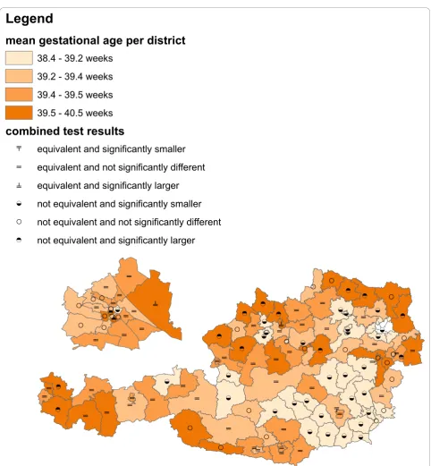
The following two examples are based on Austrian vital statistics data (source: Statistics Austria [6]) which includes all births in Austria from 1970 onwards. The Republic of Austria consists of 121 administrative dis-tricts, from which 23 (19%) constitute the densely popu-lated capital city Vienna. About 1.7 million (20%) out of about 8.4 million inhabitants live in Vienna. For the sake of better visualisation we have cut out Vienna in our choropleth maps from its location in the north-east of Austria, magnified it and placed it above the western districts (Figures 3, 4 and 5). The choropleth maps have been produced with ArcGIS 9. A significance level a= 0.05, as is customary in medicine, was used throughout the examples.

Gestational age in Austria 2008

In 2008, a total of 60,303 newborns with Austrian mothers had been recorded from where we analysed gestational age within the administrative districts. Tests for equivalence and difference were done in SAS using the procedure TTEST (option TOST for equivalence test). The equivalence range (c-Δ1,c+Δ2) was set to a

width of 4 days, i.e.Δ1 =Δ2= 2/7 = 0.286 weeks and c

was set to the sample mean x of Austrian newborns recorded from 1999 to 2007, that is, c= =x 39 4. 17

weeks.

The mean gestational ages of the districts are split at the quartiles into four categories which are represented

with different colours. Six combined scenarios of the equivalence/difference test results are represented with different symbols (Table 1). Both, colours and symbols are displayed together in one graphic (Figure 3).

The non-random spatial distribution of mean gesta-tional ages is obvious (Figure 3). In particular, shorter gestational age seems to be common in the south-eastern parts of Austria. Prolonged gestational age becomes more frequent in the north-eastern, central and western parts of Austria. The equivalence/difference testing informa-tion supports this impression (Figure 3). There is an equivalence/difference testing symbol in the opening which appeared after cutting out the capital Vienna. It belongs to a district surrounding Vienna which consists of several spatially separated areas.

Jointly displaying the variable of interest with colours and the equivalence/difference test results with symbols clearly emphasizes the former over the latter. Detailed information for specific districts can be retained on clo-ser inspection, but it is rather difficult to get an overall spatial impression of the equivalence/difference testing information from this form of graphical representation.

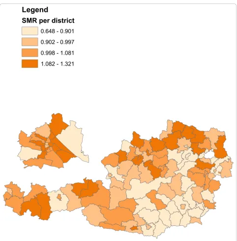
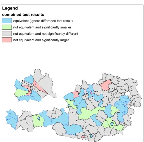
Infant mortality in Austria 1984-2007

Infant mortality (death of a live birth during the first year) was recorded between 1984 and 2007 in 121 administrative districts. A total of 10,914 out of 1,985,203 live births deceased. Inclusion criteria for the data set were that the infants had been born as single-tons between the 24th and 44th week of gestation to mothers between 13 to 50 years of age. Expected num-bers of cases per district were calculated by multiplying the national infant mortality rate with district specific numbers of births. Standardized mortality ratios were calculated as in Waldhoer et al. [7]. Equivalence and dif-ference tests were performed with the SAS macro of Daly [8]. The equivalence range (0.8, 1.25) was used.

The district SMR’s are split at the quartiles into four cate-gories and represented with different colours (Figure 4). Four combined scenarios of the equivalence/difference test results are as well represented with different colours in a separate graphic (Table 1, Figure 5).

The results of the combined equivalence/difference test results in Figure 5 only partly confirm the results of Figure 4 as more than half of the districts do not allow conclusive decisions.

Separately representing the variable of interest and the equivalence/difference test results with colours puts equal emphasis on both features which is in contrast to the colours/symbols representation of Figure 3.

Discussion and conclusions

integrating difference and equivalence test results into choropleth maps. The main aim of Figure 3 is a concise combination of the spatial distribution of the variable of interest and the statistical test results, where the focus is on the former and the latter is meant to provide supple-mentary information only. On the other hand, Figures 4 and 5 show a situation where both, data description and

statistical testing are of equal interest. It should be noted that other forms of graphical representation could be considered to effectively communicate the bivariate information [see e.g. [9-11]].

The non-random spatial distribution of infant mortal-ity in Figure 4 closely resembles that of gestational age in Figure 3. Shorter gestational age seems to be

ż

ő <

ż

ż

ż

ő

ż

ő ő ő

ż

_ő ő ő ő _ő <

ż

< <

ż

ż

< ő

ż

<

ż

< < < <

ż

ő

ż

< < < < ő

ż

ő < ő Ũ

ż

< < < ő ő ő ő ő ő

ż

< < ő < < < ő < ő <

ż

ő ő < < < < ť < < < < ő ő < < < < < ő ő ő ő < ő

ż

ő ő < < ő ő < ő ő

ż

<

ż

<

ż

ő ő ő

ż

ż

ż

ż

ő

ż ż

ő ő ő Ũ ő

Legend

mean gestational age per district

38.4 - 39.2 weeks

39.2 - 39.4 weeks

39.4 - 39.5 weeks

39.5 - 40.5 weeks

combined test results

ť

equivalent and significantly smaller

ő

equivalent and not significantly different

Ũ

equivalent and significantly larger

<

not equivalent and significantly smaller

ż

not equivalent and not significantly different

<

not equivalent and significantly larger

m

m

m

m

associated with decreased infant mortality. Drawing cau-sal relationships, however, may be fallacious for two rea-sons. Firstly, the study times do not overlap (2008 in Figure 3 and 1984-2007 in Figure 4), and secondly, there is the possibility of an ecological inference fallacy.

Figure 4 provides a rather typical example of a tradi-tional epidemiological choropleth map. The clear non-random spatial distribution in Figure 4 exhibits many districts with increased and decreased risk in the north-west and south-east of Austria, respectively. When defining a range from 0.8 to 1.25 as equivalent and

therefore not important enough to raise public health concerns, then about 40% of the districts will allow conclusive decisions (red-, green- and blue-coloured districts in Figure 5). The indefiniteness of the gray-coloured districts may be mainly due to lack of statisti-cal power, however, in any case valuable additional information for local health authorities is provided.

Both examples differ in a further small, but crucial detail. In the gestational age example, the null hypoth-esis value c is determined from a previous data set (1999 to 2007) in order to test the various districts in

Legend

SMR per district

0.648 - 0.901

0.902 - 0.997

0.998 - 1.081

1.082 - 1.321

the data set at hand (2008), and both data sets do not overlap.

In the infant mortality example, on the contrary, all live births from 1984 to 2007 were used to calculate the national infant mortality rate which, via SMR, is tested against the district infant mortality rates from 1984 to 2007. That is, the null hypothesis is partially determined by the data which are to be tested. This means that a districts rate is compared with all other district rates including its own one. Although such an approach is statistically questionable, it is quite common in spatial

epidemiology. As long as the number of cases and the size of the population of the respective district are small compared to the whole national sample, the thereby arising bias can be safely ignored. Note that there is a structurally similar problem in the field of relative survi-val where people suffering from an illness are compared to the overall population including the diseased ones.

Both examples are based on fixed effect estimators, which neither do account for spatial autocorrelation in the underlying variables nor do correct for the inherent multiplicity. It would be rather straightforward to

Legend

combined test results

equivalent (ignore difference test result)

not equivalent and significantly smaller

not equivalent and not significantly different

not equivalent and significantly larger

translate the approach to random or mixed effect mod-els with either global or local shrinkage (spatial smooth-ing) which “borrow strength” from adjacent districts. Corrections for multiple testing could be performed within the models in order to account for reduced degrees of freedom by positive spatial autocorrelation. Multiple testing will not be an explicit issue if spatial smoothing is performed within a Bayesian setting as “a correct adjustment is automatic within the Bayesian paradigm”[12].

Note that the decision for a multiplicity adjustment before reporting public health results has to consider both technical and non-technical points. Multiplicity is an issue to be kept in mind when looking from a nationwide or transregional level at a series of regio-nal test results. On the contrary, individual persons and local health authorities may only be interested in their corresponding local area results. Similar argu-ments apply for the choice between simple fixed effect and spatially smoothed estimates. There might be local health authorities, who might resist against a seeming degradation of their spotless public health records by the inclusion of ill-performing neighboring districts due to spatial smoothing. Critics from the local residents and the media might argue that shrink-age and smoothing is merely a convenient tool for understating unpleasant results, particularly, as spatial smoothing may yield essentially conservative results [13]. On the other hand, spatially smoothed results are more stable and less prone to random fluctuations. Governmental agencies interested in an overall picture may favor them.

Concluding, we think that enhancing spatial maps with a combination of statistical difference and equivalence test results could help to classify epidemiological findings the right way. A better understanding of spatial observa-tions could be achieved by explicitly defining their rele-vance through a pre-defined equivalence range. In order to apply our suggested method all is needed are confi-dence intervals or - in a Bayesian setting - credibility intervals for the small area parameters of interests. Tech-nically, it does not matter whether or not these intervals have been“preprocessed”by multiplicity adjustments or spatial smoothing.

Finally note thatequivalence anddifferencemay have other sensible meanings than those employed here. In the field of spatial epidemiology equivalence may be considered as spatial clustering and differencemay be related to spatial outliers or excessive observations. Examples of methods which address these notions of

equivalence anddifferencein combination include LISA statistics [14] and Oden’sIpop[15].

Additional material

Additional file 1: Does the joint application of a difference and an equivalence test pose a multiple testing problem? It is stated in the Multiple testing subsection that jointly performing a difference and an equivalence test for a single spatial unit maintains the multiple level of significance at_a. A formal proof for this statement is provided.

Acknowledgements

The authors thank the anonymous reviewers for helpful suggestions which improved the manuscript.

Author details 1

Department of Epidemiology, Center for Public Health, Medical University of Vienna, Borschkegasse 8a, A-1090 Vienna, Austria.2_{Center for Medical}

Statistics, Informatics, and Intelligent Systems, Medical University of Vienna, Spitalgasse 23, A-1090 Vienna, Austria.

Authors’contributions

Both authors contributed equally to this research. Both authors read and approved the final manuscript.

Competing interests

The authors declare that they have no competing interests.

Received: 16 September 2010 Accepted: 10 January 2011 Published: 10 January 2011

References

1. Sonnemann E:Allgemeine Lösungen multipler Testprobleme.EDV in Medizin und Biologie1982,13(4):120-128, English version of the original article with minor corrections by Finner H: General Solutions to Multiple Testing Problems. Biometrical Journal 2008, 50(5):641-656.

2. Hauschke D, Steinijans VW:Directional decision for a two-tailed alternative.Letter to the editor. Journal of Biopharmaceutical Statistics1996,

6(2):211-213.

3. Food and Drug Administration:Guidance for Industry. Bioavailability and Bioequivalence Studies for Orally Administered Drug Products - General Considerations.2003 [http://www.fda.gov/downloads/Drugs/

GuidanceComplianceRegulatoryInformation/Guidances/ucm070124.pdf], Revision 1.

4. Hirji KF:Exact analysis of discrete dataBoca Raton: Chapman & Hall/CRC; 2006, ISBN-13: 978-1584880707.

5. Wellek S:Testing Statistical Hypotheses of EquivalenceBoca Raton: Chapman & Hall/CRC; 2003, ISBN-13: 978-1584881605.

6. Austria Statistics:Vital statistics.[http://www.statistik.at/web_en/statistics/ population/births/index.html].

7. Waldhoer T, Wald M, Heinzl H:Analysis of the spatial distribution of infant mortality by cause of death in Austria in 1984 to 2006.

International Journal of Health Geographics2008,7:21.

8. Daly L:Simple SAS macros for the calculation of exact binomial and Poisson confidence limits.Computers in Biology and Medicine1992,22(5):351-361. 9. Carr DB, Wallin JF, Carr DA:Two new templates for epidemiology

applications: linked micromap plots and conditioned choropleth maps.

Statistics in Medicine2000,19(17-18):2521-2538.

10. Bell BS, Hoskins RE, Pickle LW, Wartenberg D:Current practices in spatial analysis of cancer data: mapping health statistics to inform

policymakers and the public.International Journal of Health Geographics

2006,5:49.

11. Pickle LW, Carr DB:Visualizing health data with micromaps.Spatial and Spatio-temporal Epidemiology2010,1(2-3):143-150.

12. Bayarri MJ, Berger JO:The Interplay of Bayesian and Frequentist Analysis.

Statistical Science2004,19(1):58-80.

14. Anselin L:Local Indicators of Spatial Association–LISA.Geographical Analysis1995,27(2):93-115.

15. Oden N:Adjusting Moran’s I for population density.Statistics in Medicine

1995,14(1):17-26.

doi:10.1186/1476-072X-10-3

Cite this article as:Waldhoer and Heinzl:Combining difference and

equivalence test results in spatial maps.International Journal of Health

Geographics201110:3.

Submit your next manuscript to BioMed Central and take full advantage of:

• Convenient online submission

• Thorough peer review

• No space constraints or color figure charges

• Immediate publication on acceptance

• Inclusion in PubMed, CAS, Scopus and Google Scholar

• Research which is freely available for redistribution