R E S E A R C H
Open Access
Adhesive joint computations using cohesive
zones
Nunziante Valoroso
1*and Silvio de Barros
2*Correspondence: nunziante. [email protected] 1Università di Napoli Parthenope,
Dipartimento di Ingegneria, Centro Direzionale Isola C4, Napoli 80143, Italy
Full list of author information is available at the end of the article
Abstract
Background: The cohesive zone approach has gained increasing success in recent years for simulating debonding and fracture via finite element methods and is ideally suited for simulating adhesive joints, the potential crack paths being generally known in advance in most cases. In the paper the determination of the size of the so-called cohesive process zone is discussed, i.e. the region wherein the stress and damage state have to be correctly resolved in order to properly quantify the dissipated energy and the load bearing capacity of the structure. An a priori estimate for the size of the active process zone is provided based on the beam on elastic foundation model in which the material parameters of the cohesive law are incorporated.
Methods: The formulation of the cohesive model in a damage mechanics format is first provided. The beam on elastic foundation model is then recalled and an
approximate solution for the cohesive zone length is found that depends on a material length and a geometric parameter as well.
Results and discussion: Numerical results are presented for a Double Cantilever Beam (DCB) geometry with varying thickness for which bilinear and exponential cohesive laws are considered. The influence of the geometry and of the shape of the cohesive law are put forward in terms of global response and evolution of the cohesive process zone. Conclusions: The size of the process zone is found to be quite sensitive to the specimen characteristic size, whose influence is well captured even using a simplified modeling wherein the original cohesive law is changed into an ideal perfectly brittle one. This leads to fairly good estimates of the size of the cohesive zone compared to finite element results.
Keywords: Adhesive joints; Cohesive zone; Interface elements
Background
Recent advances in adhesive bonding technologies have led to a rapid growth in the use of structural adhesives and in many cases their use is by far more convenient than tra-ditional joining methods [1,2]. Namely, a major advantage of structural adhesive joints is that they provide more uniform stress transfer compared to other types of fastening sys-tems; however, most adhesive bonds contain defects such as voids, regions with no or poor bonding and micro cracks, and such defects might grow under loading and give rise to local decohesion and formation of macro fractures.
To a great extent, at the onset of decohesion in a bonded joint the surface tractions between the joined adherends do not suddenly drop to zero owing to the presence of
low-range interactions that precede the formation of traction-free surfaces. Such inter-actions can be effectively described by allowing jumps in the displacement field along an interface where crack propagation is known or is expected to occur. At each point of the interface such displacement discontinuities have then to be related to surface tractions components via a decohesion model, i.e. a relationship able of representing the differ-ent phases of the potdiffer-ential debonding process from the initial undamaged condition to progressive damage and up to fracture propagation. The driving idea for such a class of models is the cohesive-zone concept initially introduced by Barenblatt [3] and Dugdale [4]. This approach has gained major popularity in recent years for simulating delami-nation, debonding, fracture and fragmentation via finite element methods and is ideally suited for simulating adhesive joints, the potential crack paths being generally known in advance in most cases, see e.g. [5,6] and references therein for recent survey accounts.
Adhesive joints may be loaded to failure in the design configurations or in the form of test specimens and it is important to fully understand the response obtained by such testing especially for the apparently simple configurations used in international standards since fracture behavior is in general governed by material properties, loading conditions and geometrical parameters as well. Moreover, apart from being employed for studying sensitivity and data reduction [7,8], simple joint configurations can be interpreted on a theoretical basis to define requirements for elements and for the mesh that guarantee meaningful answers from numerics. This is indeed a crucial point since it has a direct impact on the results of computations.
In this paper one of such critical aspects of finite element analysis of adhesive joints is discussed, i.e. the estimation of the size of the cohesive process zone. This is the region wherein the stress and damage state must be correctly resolved to properly quantify the dissipated energy and the load bearing capacity of the structure.
It is well known that a cohesive model brings a length scale into the problem in the form of a characteristic length parameter; this expresses the length over which the cohesive constitutive relation plays a role. A recent survey about length scales in the simulation of delamination and fracture can be found in [9]; worth mentioning is also Reference [10], where is provided a table comparing the different expressions proposed in the literature to estimate the cohesive zone extension.
Based on a simplified modeling, in the present work an a priori estimate for the size of the active process zone under mode-I conditions, and for the size of the nearby region subject to compressive stresses as well, is provided. To this end use is made of a beam on elastic foundation model in which the material parameters of the cohesive law are incorporated. The expressions obtained that quantify the extension of the cohesive zone are fairly accurate and very easy to implement. This is demonstrated through numerical experiments in which we consider two different shapes of the traction-separation law and simulate two symmetric double cantilever beam (DCB) fracture specimens with different characteristic geometric size.
Methods
Cohesive model
and the crack advancement. In particular, in the following we refer to the model originally presented in [11] and consider the only one-dimensional (mode I) case, that is governed by the following equations:
t=(1−D)k[[u]]++k−[[u]]− Y= 12k[[u]]2+
Y−F(D)≤0; D˙ ≥0; D˙(Y−F(D))=0
(1)
In the above relationshipst andY respectively denote the interface traction and the damage-driving force,D ∈[ 0, 1] is the scalar damage variable, [[u]] is the displacement jump in the direction normal to the interface,·±indicates the positive (negative) parts of the argument whilekandk−are the undamaged interface stiffness parameters in tension and compression, respectively.
Damage irreversibility is enforced by requiring that the critical damage-driving force cannot decrease; therefore, its value can be determined by a monotonically increasing positive functionF, typically a power law or an exponential, whose explicit expression is constructed in a way to ensure that the energy dissipated in the formation of a new unit traction-free surface equals the adhesive fracture energyGc. In particular, the exponential
traction-separation relationship given in [11] can be obtained using:
Fe(D)=Go−(Gc−Go)log(1−D) (2)
whereas the widely used bilinear cohesive law with finite initial stiffness follows from the damage function:
Fb(D)=
G2cGo
[GoD+Gc(1−D)]2
(3)
We emphasize that the formulation at hand requires no time-integration for computing the damage state, that can be evaluated explicitly. In particular, for damage loading (D˙ > 0) at each timeτ the damage variable can be obtained as:
D(τ )=min
1, max (σ≤τ ){F
−1(Y(σ ))}
(4)
Beam on elastic foundation model
The idea of using the beam on elastic foundation model to analyze adhesively bonded specimens is not new. In earlier applications it has been employed in the form of the one-parameter Winkler model to compute corrections factors for the DCB specimen for data reduction based on beam theories [12], see also [13].
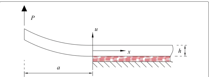
The formulation of the basic Winkler model can be found in classical textbooks in Mechanics, see e.g. [14], and will not be repeated here. Referring to Figure 1 for the geom-etry and symbols relevant to the cantilever beam under consideration, for the case at hand the deflection for the bonded regionx>0 can be expressed as:
u(x)=exp(−λx)·[Acos(λx)+Bsin(λx)] (5)
whereλis the reciprocal of the model wavelength given as:
1 λ=
Eh3 3k
1
4
(6)
Figure 1 Cantilever beam on elastic foundation model of the adhesive joint.
distributed load. The parameter (6) has the dimensions of a length that results from the product of a material length and a geometric dimension. Actually, the interface elastic stiffness ratioE/kis proportional to the characteristic length parameter of the cohesive law provided in [15] as:
lc=
E Gc
t2
max
(7)
whereby one has: 1
λ4 ∝lc·h
3 (8)
ConstantsAandBin Equation (5) are computed from boundary conditions. Their sim-plest expression is obtained using the boundary conditions on the shear force and the bending moment atx=0 to get:
A= −1 2
Pa
EIλ2; B= 1 2
P(1+λa)
EIλ3 (9)
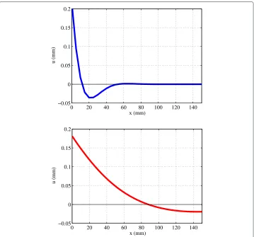
Typical plots of the beam deflection (5) are given in Figure 2, where are depicted the solutions of a thin and of a moderately thick beam, respectively.
In particular, Figure 2 suggest that a way to quantify the size of the cohesive zone in a DCB specimen is to use (5), and in particular to use the roots of the equationu(x) = 0 that, on account of (9), can be expressed as:
xn=
1 λ
arctan
1+λa λa
+nπ
(10)
for integersn≥ 0. Relationship (10) applies provided that the constitution of the inter-face is linear. An approximate solution for a nonlinear interinter-face model can however be obtained by changing the shape of the cohesive relationship into a virtually perfectly brit-tle law that preserves either the interface stiffnesskor the peak stresstmaxof the nonlinear
law. In the first case the beam length parameter has the expression (6) and the maximum stress of a brittle law with the same fracture energy increases to the value
tmax=
2kGc (11)
In the second case, to keep the peak stress fixed for given critical fracture energy the characteristic length is expressed as function of the cohesive properties as:
1 λ =
2 3
EGch3
t2
max
1
4
0 20 40 60 80 100 120 140 −0.05
0 0.05 0.1 0.15 0.2
u (mm)
x (mm)
0 20 40 60 80 100 120 140
−0.05 0 0.05 0.1 0.15 0.2
u (mm)
x (mm)
Figure 2 Beam deflection forλ−18mm(top) andλ−150mm(bottom).
and the interface stiffness of the elastic foundation model takes the (reduced) value
k= t
2
max
2Gc
(13)
In closing this section we remind that, apart from the factor(2/3)1/40.9, the expres-sion (12) is usually taken to represent the length of the cohesive damage zone in slender composite laminates [16].
Results and discussion
The cohesive model summarized in the previous Section has been implemented in a cus-tomized version of the finite element code FEAP [17]. For the computations described in this section use has been made of enhanced assumed strain quadrilaterals for the bulk material and 4-noded interface elements.
As a numerical example we refer to the classical DCB geometry under plane strain conditions. Loading is simulated via displacement control and either a bilinear or an expo-nential cohesive law are considered. For results to be comparable the same critical fracture energyGc =0.125 N/mm and peak stresstmax =10 N/mm2have been taken as
initial flaw isa=50 mm and the arm height is taken ash=8 mm for the thin beam and h = 80 mm for the thick case. Unlike the thin beam, which corresponds to the geom-etry that has been experimentally tested in [5], the thick beam case is a pure numerical exercise aiming to reproduce a stiff structure for which the size of the cohesive zone is comparable to the dimensions of the sample, see also [18].
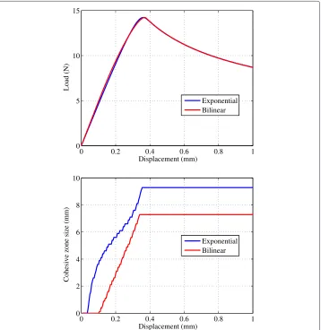
Figure 3 shows the solution for the thin DCB in terms of global load-deflection curve and size of the cohesive zone. As for the load-deflection curve, no substantial difference appears between the responses obtained with the two different cohesive laws, that yield practically coincident results at the global level. Contrariwise, the sizelcohof the cohesive
process zone is found to be more sensitive to the shape of the cohesive law. In both exam-ined cases, a steady state is attaexam-ined for a load level close to the peak load and using finite element analysis the size of the damage cohesive zone is found to belcoh,exp = 9.28 mm
for the exponential cohesive law andlcoh,bil=7.23 mm for the bilinear one.
From the beam on elastic foundation model the size of the cohesive zone follows from relationship (10) forn=0, i.e. as the first zero of the deflection function (5), whereby one obtains a lengthx0 = 11.8 mm when using the stiffness-preserving wavelength (6) and
x0 = 6.31 mm when expression (12) is adopted instead. The interval defined by these
0 0.2 0.4 0.6 0.8 1
0 5 10 15
Load (N)
Displacement (mm)
Exponential Bilinear
0 0.2 0.4 0.6 0.8 1
0 2 4 6 8 10
Displacement (mm)
Cohesive zone size (mm)
Exponential Bilinear
values clearly delimits the length of the damage cohesive zone computed via finite ele-ments whereas the material length parameter defined in (7) is computed aslc=87.5 mm,
which is quite far from the numerical solution. As for the size of the region subject to com-pressive stresses ahead of the crack front, from finite element computations one obtains a length of about 30 mm while from (10) one obtainsx1−x0=π/λ ∈[ 25.6, 41.3] mm, which again includes the numerically computed value.
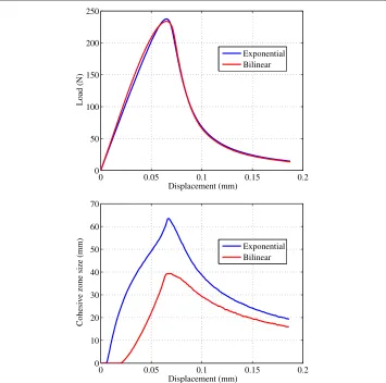
In the second series of computations the only thicknesshof the arms of the DCB is increased from 8 mm to 80 mm while material properties are kept the same as for the thin specimen. In this case the differences in the computed solutions obtained with the two cohesive models are more apparent for both the load-deflection curves and the extension of the cohesive zone, see Figure 4.
For the case at hand of the thick specimen, no steady state is reached in the evolution of the cohesive zone size that starts decreasing right after the peak load has been attained. The maximum length for the damage cohesive zone computed via finite element analysis is found to belcoh,exp=63.5 mm for the exponential cohesive law andlcoh,bil=39.2 mm
for the bilinear one whereas from the Winkler model the size of the cohesive zone is estimated either asx0= 44.5 mm if the wavelength is computed using (6) or asx0= 87.8 mm when referring to (12). Obviously, the length parameter (7) is the same as before
0 0.05 0.1 0.15 0.2
0 50 100 150 200 250
Load (N)
Displacement (mm)
Exponential Bilinear
0 0.05 0.1 0.15 0.2
0 10 20 30 40 50 60 70
Displacement (mm)
Cohesive zone size (mm)
Exponential Bilinear
since, by definition, it is independent from the specimen size. As for the size of the region subject to compressive stresses ahead of the crack front, it is numerically found to extend up to the right free end of the specimen. This is confirmed from (10) as well, whereby it is estimated asx1−x0=π/λ ∈[ 130.6, 232.2] mm, which practically exceeds the specimen length.
Based on the previous results one could conclude that the size of the cohesive process zone is captured fairly well for both the thin and thick DCB cases, which demonstrates the importance of using an estimate that includes a geometric parameter in addition to the material length scale (7). Despite the intrinsic limitations of the adopted simplified modeling, that basically relies upon linear elastic considerations, the a priori estimates for the size of both the cohesive zone and of the compressed region ahead of the crack front seem to be reliable especially for the thin DCB case. On the contrary, for the thick DCB a priori estimates do not compare well as in the previous case; this is likely to occur because for the thick DCB the cohesive zone is not completely developed since the beam cannot be considered long compared to the model wavelength.
Conclusions
A simplified modeling for estimating the cohesive zone size in mode-I debonding prob-lems across a range of geometrical properties has been presented. In particular, it is shown that the size of the damaged zone and that of the region subject to compressive stresses ahead of the crack front can be estimated with good approximation as functions of the cohesive parameters and of the specimen geometry via a beam on elastic founda-tion model. Unlike the global load-deflecfounda-tion response, for a given characteristic length of the traction-separation law the size of the process zone is found to be quite sensitive to the specimen characteristic size, whose influence is well captured even using a simplified modeling.
In the present paper comparisons between finite element results and the beam model have been carried out by modifying the shape of the cohesive law in a way to preserve either the initial stiffness or the peak stress. This has led to fairly good estimates of the size of the cohesive zone. In the Authors’ opinion the subject is worth investigating and alternative strategies to improve the predictive capabilities of the present approach will be examined in forthcoming papers.
Competing interests
The authors declare that they have no competing interests.
Authors’ contributions
NV designed the methodologies and wrote the paper. SDB collected and summarized the data. Both authors have read and approved the final manuscript.
Author details
1Università di Napoli Parthenope, Dipartimento di Ingegneria, Centro Direzionale Isola C4, Napoli 80143, Italy.2Centro Federal de Educação Tecnológica, Departamento de Engenharia Mecânica, Av. Maracanã, 229 - Bloco E 5o andar, Rio de Janeiro 20271-110, Brasil.
Received: 4 October 2013 Accepted: 3 December 2013 Published: 30 December 2013
References
1. Adams RD (2005) Adhesive Bonding: Science, Technology and Applications. CRC Press, Boca Raton 2. da Silva LFM, Ochsner A, Adams RD (eds) (2011) Handbook of adhesion technology. Springer, Heidelberg 3. Barenblatt GI (1962) The Mathematical Theory of Equilibrium Cracks in Brittle Fracture. In: Dryden HL, von Kármán Th,
4. Dugdale DS (1960) Yielding of steel sheets containing slits. J Mech Phys Solids 8(2): 100–104
5. Valoroso N, Sessa S, Lepore M, Cricrì G (2013) Identification of mode-I cohesive parameters for bonded interfaces based on DCB test. Eng Fracture Mech 104(1): 56–79
6. Campilho RDSG, Banea MD, Neto JABP, da Silva LFM (2013) Modelling adhesive joints with cohesive zone models: effect of the cohesive law shape of the adhesive layer. Int J Adhesion Adhesives 44: 48–56
7. Valoroso N, Fedele R (2010) Characterization of a cohesive-zone model describing damage and de-cohesion at bonded interfaces: sensitivity analysis and mode-I parameter identification. Int J Solids Struct 47(13): 1666–1677 8. Fedele R, Sessa S, Valoroso N (2012) Image correlation-based identification of fracture parameters for structural
adhesives. Technische Mech 32(2): 195–204
9. Harper PW, Hallett SR (2008) Cohesive zone length in numerical simulations of composite delamination. Eng Fracture Mech 75(16): 4774–4792
10. Turon A, Dávila CG, Camanho PP, Costa J (2007) An engineering solution for mesh size effects in the simulation of delamination using cohesive zone models. Eng Fracture Mech 74(10): 1665–1682
11. Valoroso N, Champaney L (2006) A damage-mechanics-based approach for modelling decohesion in adhesively bonded assemblies. Eng Fracture Mech 73(18): 2774–2801
12. Williams JG (1989) End corrections for orthotropic DCB specimens. Composites Sci Technol 35(4): 367–376 13. Williams JG, Hadavinia H (2002) Analytical solutions of cohesive zone models. J Mech Phys Solids 50(4): 809–825 14. Timoshenko SP, Goodier JN (1970) Theory of elasticity, 3rd edn. McGraw Hill, Singapore
15. Hillerborg A, Modéer M, Petersson P-E (1976) Analysis of crack formation and crack growth in concrete by means of fracture mechanics and finite elements. Cement Concrete Res 6(6): 773–781
16. Yang Q, Cox B (2005) Cohesive models for damage evolution in laminated composites. Int J Fracture 133(2): 107–137 17. Taylor RL (2013) FEAP - Programmer Manual. http://www.ce.berkeley.edu/projects/feap/pmanual84.pdf
18. Alfano G, de Barros S, Champaney L, Valoroso N (2004) Comparison between two cohesive-zone models for the analysis of interface debonding. In: Neittaanmäki P, Rossi T, Majava K, Pironneau O (eds) European Congress on Computational Methods in Applied Sciences and Engineering. University of Jyväskylä, Department of Mathematical Information Technology, Finland
doi:10.1186/2196-4351-1-8
Cite this article as:Valoroso and de Barros:Adhesive joint computations using cohesive zones.Applied Adhesion Science
20131:8.
Submit your manuscript to a
journal and benefi t from:
7Convenient online submission
7Rigorous peer review
7Immediate publication on acceptance
7Open access: articles freely available online
7High visibility within the fi eld
7Retaining the copyright to your article