New parameter of roundness R: circularity corrected by aspect ratio

M E T H O D O L O G Y

Open Access

New parameter of roundness

R: circularity

corrected by aspect ratio

Yasuhiro Takashimizu

and Maiko Iiyoshi

Abstract

In this paper, we propose a new roundness parameter_R, to denote circularity corrected by aspect ratio. The basic concept of this new roundness parameter is given by the following equation:

R= Circularity + (Circularityperfect circleCircularityaspect ratio)

where Circularityperfect circleis the maximum value of circularity and Circularityaspect ratiois the circularity when only the aspect ratio varies from that of a perfect circle. Based on tests of digital circle and ellipse images using ImageJ software, the effective sizes and aspect ratios of such images for the calculation ofRwere found to range between 100 and 1024 pixels, and 10:1 to 10:10, respectively._Ris thus given by

R= CI+ (0.913−CAR)

where CIis the circularity measured using ImageJ software and CARis the sixth-degree function of the aspect ratio measured using the same software. The correlation coefficient between the new parameter_Rand Krumbein’s roundness is 0.937 (adjusted coefficient of determination = 0.874). Results from the application ofRto modern beach and slope deposits showed thatRis able to quantitatively separate both types of material in terms of roundness. Therefore, we believe that the new roundness parameter_Rwill be useful for performing precise statistical analyses of the roundness of particles in the future.

Keywords:Aspect ratio, Circularity, ImageJ software, Krumbein’s visual roundness, Roundness

Background

Many studies have investigated particle shape in the natural world, mostly based on the definitions of sphericity and roundness of rock particles proposed by Wadell (1932). Previous studies into particle shape have been discussed in a series of review arti-cles (e.g., Barrett 1980; Clark 1981; Winkelmolen 1982; Diepenbroek et al. 1992; Blott and Pye 2008), and in general, such studies have mainly taken one of two approaches to understanding particle shape. The first is a simple method that involves the exam-ination of visual images of particle grains (e.g., Krumbein 1941; Rittenhouse 1943; Powers 1953; Pettijohn 1957; Lees 1963). Determining roundness using the visual roundness chart proposed by Krumbein, which is further extended in this paper, is one of the most widely employed methods. However, such a method merely compares visual images, and therefore, the derived roundness values are

not strictly quantitative. The second approach involves the quantitative determination of various shape parame-ters, and many evaluation methods have been designed to obtain relevant shape parameters (e.g., Schwarcz and Shane 1969; Orford and Whalley 1983; Diepenbroek et al. 1992; Yoshimura and Ogawa 1993; Vallejo and Zhou 1995; Bowman et al. 2001; Itabashi et al. 2004; Drevin 2007; Blott and Pye 2008; Lira and Pina 2009; Roussillon et al. 2009; Arasan et al. 2011; Suzuki et al. 2013, 2015). Both approaches, however, involve the analysis of each individual particle, and therefore, production of several thousand to several tens of thousands of shape parameters for reliable analysis is time consuming. Therefore, owing to the extensive time requirements and effort required for both approaches, neither is widely used, and there remains a need for an easy statistical method to derive parameters of particle shape.

In this study, we define a new roundness parameter, R, to denote the circularity corrected by aspect ratio, and present a case study of R calculation using ImageJ software (ver. 1.47q) released from the US National * Correspondence:[email protected]

1_{Faculty of Education, Niigata University, Niigata 950-2181, Japan} Full list of author information is available at the end of the article

Institute of Health (Abramoff et al. 2004; Schneider et al. 2012). This represents a fairly simple method that helps to overcome the shortcomings of the previously published methods discussed above.

Basic concept of this study

The proposed concept for the new roundness par-ameter is quite simple: It is a correction of circu-larity using the aspect ratio of particles. The definition of circularity, corresponding to that of parameter K defined by Cox (1927), is given as follows:

Circularity ¼4π⋅ Area

Perimeter2 ð1Þ

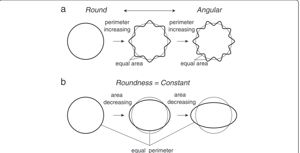
This indicates that circularity can be altered in two ways: by changes in area and by changes in the perim-eter of a particle. To consider this, an ideal perfect circle (true circle) is assumed. If the area and perimeter do not change, then circularity is constant. However, if only the perimeter increases and the area does not change (Fig. 1a, towards the right), then circularity de-creases. An increase in the perimeter length there-fore represents a decrease in the roundness of the particle. It should be noted that in this paper, we use the term “roundness” to refer to the presence or absence of surface irregularities. Therefore, with a

decrease in roundness, circularity also decreases. In comparison, in the case of the ellipses skewed from a circle, if only the area decreases and the perimeter does not change, then circularity can also be seen to decrease (Fig. 1b). A decrease in area in this way represents an increase in the aspect ratio of the par-ticle image. Therefore, with a increase in the aspect ratio, the circularity also decreases. In Fig. 1b, how-ever, the transformed images in the center and on the right still show a high degree of roundness. Consequently, it should be possible to determine roundness if circularity can be corrected using aspect ratio. In other words, if it is possible to combine the difference in circularity value due to aspect ratio with the circularity itself, then the aspect ratio-corrected circu-larity can be used to represent roundness. Thus, our roundness parameterRcan be defined by the following equation:

R¼Circularityþ Circularityperfect circle−Circularityaspect ratio

ð2Þ

where Circularity is the value defined by Eq. (1), Circularityperfect circle is the maximum value of circu-larity, and Circularityaspect ratiois the circularity when only the aspect ratio varies from that of a perfect circle.

equal area

Round

Angular

perimeter increasing

Roundness = Constant

area decreasing

equal area

equal perimeter perimeter increasing

area decreasing

a

b

Fig. 1Basic concept of transformation from a perfect circle.Narrow solid linesdenote perfect circles before transformation.aOnly the perimeter increases; the area does not change.bOnly the area decreases; the perimeter does not change

Case study of parameterRcalculation using ImageJ software

In this chapter, we present a specific case study, demon-strating the calculation of the parameterRdefined in the previous chapter, using ImageJ software.

Methods

Test digital images were produced using Adobe Photo-shop CS4 and Adobe Illustrator CS4. Shape parameters, including area, perimeter, circularity, aspect ratio, major axis length, and minor axis length, were measured from the test digital images using ImageJ software (ver. 1.47q). To validate the effectiveness of R defined in this paper, digital images of Krumbein’s original visual images (Krumbein 1941) were captured using a Fuji Xerox ApeosPort-IV C7780 scanner with a resolution of 600 × 600 dots per inch and a grayscale color profile; they were saved in a TIF image file format.

Grain-size distributions of modern slope and beach sediments were measured using a sieve ranging from

−5.0 to 4.0 phi, with 0.5 phi intervals. The first quartile (twenty-fifth percentile), second quartile (median), and third quartile (seventy-fifth percentile) of grain size were obtained for each from the cumulative curves.

To obtain the new roundness parameter R value for these modern slope and beach sediments, we used an Olympus TG-1 digital camera to acquire digital images of particles in each grain-size class. Image analysis was

then conducted separately for each grain-size fraction. The measurement of grain sizes in this analysis ranged from values equal to or coarser than 1.0 phi, with 0.5 phi intervals, with the finer limit (1.0 phi) of the measurement range determined by the limitations of the Olympus TG-1. This range was sufficient for comparing the sediments in this study, because of the coarseness of the material. For imaging, the particles were laid out on a transparent board. As the minorc-axes of the particles in this layout were nearly perpendicular to the board, we assumed that an imaginary plane perpendicular to the c-axis, which included the major and intermediate a- and b-axes, respectively, was parallel to the board. To obtain sharp silhouettes of particles, the light source was placed on the opposite side of the digital camera, allowing intentional capture of backlit images. The major lengths of the silhouettes were then adjusted to be more than 100 pixels. The digital images taken by Olympus TG-1 were transferred to the ImageJ software and processed into binary images. The circularity and aspect ratio of the silhouettes in the digital binary im-ages were then measured using the ImageJ software, and theRvalues were obtained using Eq. (8) described below. The obtained R values for each grain-size class were integrated into a totalRdistribution for the individ-ual samples using the weight percent of each grain size class. The calculated R distributions thus ranged from 0.400 to 0.925 with 0.025 intervals. The first quartile,

1448 pixels

16

23 11 8

6 4

3 2

1 pixel 64

45 32

91

362 256 181

128

512

1024 pixels

724 pixels

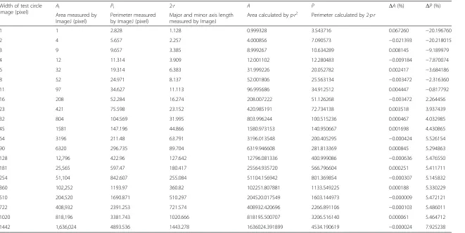
Table 1Results of error of area and perimeter for various sizes of test circle images Width of test circle

image (pixel)

AI PI 2·r A P ΔA(%) ΔP(%)

Area measured by ImageJ (pixel)

Perimeter measured by ImageJ (pixel)

Major and minor axis length measured by ImageJ

Area calculated byp·r2 _{Perimeter calculated by 2·}

p·r

1 1 2.828 1.128 0.999328 3.543716 0.067260 −20.196760

2 4 5.657 2.257 4.000856 7.090573 −0.021393 −20.218015

3 9 9.657 3.385 8.999267 10.634289 0.008145 −9.189979

4 12 11.314 3.909 12.001102 12.280483 −0.009184 −7.870074

6 32 19.314 6.383 31.999226 20.052782 0.002417 −3.684186

8 52 24.971 8.137 52.001806 25.563134 −0.003472 −2.316360

11 97 34.627 11.113 96.995686 34.912512 0.004447 −0.817792

16 208 52.284 16.274 208.007222 51.126268 −0.003472 2.264456

23 421 75.598 23.152 420.985191 72.734138 0.003518 3.937439

32 804 104.569 31.995 803.996244 100.515236 0.000467 4.032985

45 1581 147.196 44.866 1580.973153 140.950667 0.001698 4.430865

64 3196 211.48 63.791 3196.013548 200.405295 −0.000424 5.526154

90 6320 296.735 89.704 6319.946608 281.813369 0.000845 5.294863

128 12,796 422.96 127.642 12796.081336 400.999086 −0.000636 5.476550

181 25,565 597.47 180.417 25564.935720 566.796604 0.000251 5.411711

254 51,104 842.607 255.084 51104.156942 801.369854 −0.000307 5.145832

360 102,252 1193.97 360.82 102251.807881 1133.549225 0.000188 5.330229

510 204,520 1690.871 510.297 204520.017549 1603.144973 −0.000009 5.472121

722 408,932 2391.253 721.574 408932.420696 2266.891106 −0.000103 5.486011

1020 818,196 3381.743 1020.666 818195.500707 3206.516140 0.000061 5.464712

1442 1,636,024 4893.536 1443.278 1636024.391899 4534.190619 −0.000024 7.925238

p= 3.141592

Takashim

izu

and

Iiyoshi

Progress

in

Earth

and

Planetary

Science

(2016) 3:2

Page

4

of

0.000001 0.00001 0.0001 0.001 0.01 0.1 1 10 100

1 10 100 1000 10000

Error (%)

Width of digital circle image (pixel)

-1 64 pixels 1024 pixels

-1

Fig. 3Plot of the diameter of a digital circle image (pixels) and error (%) in the area and perimeter estimations

1448 pixels

1 pixel AR = 10

10

AR = 10 9

AR = 10 8

AR = 10 7

AR = 10 3

AR = 10 2

AR = 10 1 AR = 10

4 AR = 10

5 AR = 10

6

median, and third quartile of R were calculated using Microsoft Excel 2007 software.

Validation of the effective resolution of digital images using ImageJ software

A digital image is an aggregate of pixels, which are the minimum units of the image. Hence, there should be an error in shape parameter values between the geometric-ally obtained true values and those calculated from the digital image. Therefore, to obtain the most effective size of digital images for shape analysis, we examined the er-rors in basic shape parameters, including area, perimeter, and aspect ratio, using ImageJ software.

Area and perimeter

First, the area (AI), perimeter (PI), and major and minor axis lengths of the fit ellipses (2·r; both lengths are equal) of twelve test circle images with diameter lengths of 1 to 21 pixels, produced using Adobe Photoshop CS4, were calculated using ImageJ software (Fig. 2). To calculate the area and perimeter, the measuring algorithms of the ImageJ software were sought from the manual. However, there were no detailed descriptions of the algorithms, so we investigated the value determinations ourselves. The obtained algorithms are therefore as follows.AIis equal to the total number of pixels in a grain. For test circle images with a diameter length of 1 to 2 pixels,PIwas calculated by determining the geometric mean of the numbers of pixels in the images and the numbers of circumscribed pixels in the images. In contrast, for test circle images with diameter lengths greater than 2 pixels,PIwas the sum of

the marginal pixels, in which the sizes of pixels located at the corners are assumed to be 20.5, while those of other pixels is 1. The major axis length of the test circle images was 2·r, because all of the test images comprised perfect circles. The error (ΔA) between the area measured using ImageJ software (AI) and the area calculated from radius length (A), and the error (ΔP) betweenPIand the perim-eter obtained by the geometric procedure (P), were there-fore determined as follows (Table 1):

ΔA¼ AI−_AA

100 ð3Þ

ΔP¼ PI−P

P

100 ð4Þ

From our calculations, the absolute error for the area (|ΔA|) was found to decrease with an increase in the diameter of the test circle images (Table 1 and Fig. 3). All 21 |ΔA| values obtained in this test were below 0.1 %, which is sufficiently small to assume accuracy. These values are therefore sufficiently reliable for use in shape analysis. In contrast, the absolute perimeter error |ΔP| was approximately 20 % for diameters of 1 to 2 pixels, but decreased with an increase in the diameter of the test circle images. |ΔP| attained a minimum of approximately 0.8 % at a diameter of 11 pixels; however, the error increased again to approximately 8 % for diameters of 16 to 1442 pixels. For diameters of 64 to 1024 pixels, the |ΔP| value remained constant at around 5 % (Table 1 and Fig. 3).

1 10

1 10 100 1000

AR

I

Width of test ellipse image (pixel)

10 : 1 10 : 2 10 : 3 10 : 4 10 : 5 10 : 6 10 : 7 10 : 8 10 : 9 10 : 10

True aspect ratio

Fig. 5Plot of the diameter of a digital circle image (pixels) and the aspect ratio calculated using ImageJ (ARI)

Aspect ratio

In this section, we examine the relationship between the aspect ratio measured using ImageJ software (ARI) and the widths of test ellipse images (Fig. 4), which were ob-tained by subjecting the test circle images in Fig. 2 to 10 % aspect ratio deformation intervals in Adobe Photo-shop CS4. The ImageJ software defines the aspect ratio as follows:

ARI¼

major axis length of approximate ellipse minor axis length of approximate ellipse ð5Þ

Therefore, the aspect ratio is equal to one for a perfect circle and increases with an increase in deformation. To validate this relationship for different image sizes, we prepared test circle images with diameters of 20–10.5(1 to 1448) pixels, and test ellipse images were obtained from

100

pixels

10:10

10:9.1

10:1

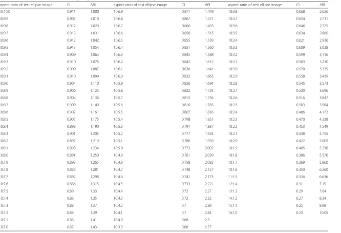
Table 2CI and ARI values calculated using ImageJ applied to the test images of Fig. 6

aspect ratio of test ellipse image CI ARI aspect ratio of test ellipse image CI ARI aspect ratio of test ellipse image CI ARI

10:10.0 0.911 1.000 10:6.9 0.871 1.449 10:3.8 0.668 2.626

10:9.9 0.905 1.010 10:6.8 0.867 1.471 10:3.7 0.654 2.711

10:9.8 0.912 1.020 10:6.7 0.860 1.493 10:3.6 0.646 2.775

10:9.7 0.913 1.031 10:6.6 0.856 1.515 10:3.5 0.634 2.860

10:9.6 0.912 1.042 10:6.5 0.855 1.539 10:3.4 0.621 2.936

10:9.5 0.913 1.054 10:6.4 0.851 1.560 10:3.3 0.609 3.038

10:9.4 0.909 1.064 10:6.3 0.845 1.588 10:3.2 0.599 3.116

10:9.3 0.910 1.075 10:6.2 0.842 1.612 10:3.1 0.583 3.230

10:9.2 0.909 1.087 10:6.1 0.836 1.641 10:3.0 0.570 3.335

10:9.1 0.910 1.099 10:6.0 0.832 1.665 10:2.9 0.558 3.439

10:9.0 0.904 1.110 10:5.9 0.826 1.694 10:2.8 0.545 3.573

10:8.9 0.906 1.123 10:5.8 0.822 1.724 10:2.7 0.530 3.696

10:8.8 0.904 1.136 10:5.7 0.815 1.756 10:2.6 0.516 3.847

10:8.7 0.909 1.149 10:5.6 0.810 1.785 10:2.5 0.503 3.984

10:8.6 0.902 1.161 10:5.5 0.807 1.816 10:2.4 0.486 4.172

10:8.5 0.905 1.175 10:5.4 0.798 1.851 10:2.3 0.470 4.338

10:8.4 0.898 1.190 10:5.3 0.791 1.887 10:2.2 0.453 4.549

10:8.3 0.901 1.205 10:5.2 0.777 1.924 10:2.1 0.438 4.755

10:8.2 0.897 1.219 10:5.1 0.780 1.959 10:2.0 0.422 5.009

10:8.1 0.898 1.234 10:5.0 0.773 2.002 10:1.9 0.405 5.236

10:8.0 0.891 1.250 10:4.9 0.761 2.039 10:1.8 0.386 5.570

10:7.9 0.893 1.265 10:4.8 0.758 2.082 10:1.7 0.369 5.860

10:7.8 0.886 1.281 10:4.7 0.748 2.127 10:1.6 0.350 6.260

10:7.7 0.892 1.298 10:4.6 0.741 2.173 11:1.5 0.334 6.636

10:7.6 0.886 1.315 10:4.5 0.733 2.221 12:1.4 0.31 7.15

10:7.5 0.89 1.33 10:4.4 0.72 2.27 13:1.3 0.29 7.64

10:7.4 0.88 1.35 10:4.3 0.72 2.32 14:1.2 0.27 8.34

10:7.3 0.88 1.37 10:4.2 0.7 2.38 15:1.1 0.25 8.98

10:7.2 0.88 1.39 10:4.1 0.7 2.44 16:1.0 0.23 10.05

10:7.1 0.88 1.41 10:4.0 0.68 2.5

10:7.0 0.87 1.43 10:3.9 0.68 2.57

Takashim

izu

and

Iiyoshi

Progress

in

Earth

and

Planetary

Science

(2016) 3:2

Page

8

of

the test circle images through 10 % deformation intervals in height (Fig. 4). As such, ARIshowed a range of values,

controlled by the widths of the test circle/ellipse images (Fig. 5). Notably, the test circle/ellipse images with di-ameters or widths of less than 100 pixels are unstable, as shown in Fig. 5. However, the widths of the test circle/ ellipse images greater than or equal to 100 pixels can be seen to remain constant.

Effective size range of digital images in this study

The above results can be summarized as follows: (1) The |ΔA| values are sufficiently small to assume accuracy for all test circle images with diameters ranging from 1 to 1442 pixels; (2) The |ΔP| value is constant, at approxi-mately 5 %, for test circle images with diameters of 64 to 1024 pixels; and (3) The ARIvalue for the test circle/ ellipse images with widths greater than or equal to 100 pixels, and a true aspect ratio greater than or equal

to 10:1, remains constant. Consequently, in this paper, we consider the effective size and aspect ratios of digital im-ages for shape analysis using ImageJ software, to be 100 to 1024 pixels and 10:1 to 10:10, respectively.

Relationship between aspect ratio and circularity in ImageJ software

Circularity in ImageJ software

Circularity can be calculated as a shape parameter index in the ImageJ software. The definition of circularity (CI) in the ImageJ software is as follows:

CI ¼ 4π⋅_PAI

I2 ð

6Þ

where AI and PI are the area and perimeter measured using ImageJ (ImageJ User 2012), respectively. This there-fore implies that CI is directly determined byAI and PI. For instance, if their two different PIvalues are provided

Fig. 7Plot of ARIandCIvalues of the test images, calculated using ImageJ software.Solid linerepresents a sixth-degree polynomial

for digital images with the same AI values, the image showing high circularity will have a shorter perimeter than that of the other image.

Relationship between circularity and aspect ratio in ImageJ software

When considering roundness as a shape parameter, the degree of roundness of a deformed circle (ellipse) image should be the same as that of a perfect circle image. Different values of CI will therefore correspond to changes in aspect ratio, and CI alone should not be used as a roundness shape parameter. For this reason, the relationship between CI and ARI is exam-ined in this section, and we attempt to correct CI using ARI.

First, a test circle image with a diameter of 100 pixels was produced using Adobe Illustrator CS4. Then, 91 test ellipse images were obtained by deforming a test circle image, in 0.1 % height intervals (Fig. 6). From the shape analysis of circularity and aspect ratio using ImageJ soft-ware, the triadic relationship between the true aspect ratio, CI, and ARI could be obtained (Table 2). ARI versusCIis plotted in Fig. 7. It should be noted that the maximum CI value is 0.913 (Table 2), as ImageJ is unable to output 1.0 as a maximum value for these test images, because the digital images comprise an aggre-gate of pixels and include errors. We used a polynomial regression to analyze the relationships. From this analysis, a sixth-degree polynomial was obtained for the relationship, with a strong correlation (r= 0.999836119, p< 0.005, adjusted coefficient of determination =

0.999648855; solid curve in Fig. 7). Thus, the estimated regression equation for the survey line is

CI¼0:826261þ0:337479ARI−0:335455ARI2

þ0:103642ARI3−0:0155562ARI4

þ0:00114582ARI5−0:0000330834ARI6

ð7Þ

where CIis the circularity calculated using ImageJ soft-ware and ARIis the aspect ratio calculated using the same software. This indicates thatCIis a sixth-degree polyno-mial of ARIwhen test ellipse images are made from the deformation of a perfect circle image with 0.1 % intervals in height. We therefore refer to theCIvalue newly derived from this regression equation asCAR.

Calculating roundness parameter R using ImageJ software Equation (7) implies that the circularity of a perfect circle changes with varying aspect ratio. This means that if a shape’s perimeter is highly rounded, then the degree of roundness should also be close to 0.913. Therefore, after the correction of circularity by aspect ratio, which represents the addition of the difference between 0.913 and CAR to CI, it is possible to calcu-late the circularity without considering aspect ratio. The corrected circularity is therefore considered the new roundness parameter (R) and can be presented as follows:

R¼CIþð0:913−CARÞ ð8Þ When using R in particle shape analysis, the round-ness values can be easily handled as numerical data.

Fig. 9Location of the study area.aLarge-scale map of study area in Northeastern Japan and facing the Pacific Ocean.bDetailed map with sampling location in the Masaki area of Iwate Prefecture, Northeastern Japan. Location map is based on“Taro,”the 1:25,000 topographic map from the Geographical Survey Institute (GSI) of Japan.Solid circleandsolid squareindicate beach and slope deposits, respectively

For instance, the first quartile (twenty-fifth percentile), second percentile (median), and third quartile (sev-enty-fifth percentile) of the roundness of a large number of particle grains can be easily and quickly examined.

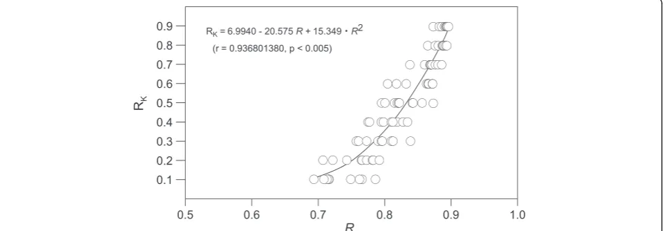
Validation ofRusing Krumbein’s pebble images for visual roundness

In order to validate the effectiveness ofRdefined in this paper, theRvalues of Krumbein’s visual images were calcu-lated and examined. Figure 8 plots Krumbein’s roundness

a

b

c

d

e

f

(R_K) against the R values calculated using the method defined in this study. From this analysis, a second-degree polynomial was obtained for the relationship, with strong correlation (r= 0.936801380,p< 0.005; adjusted coefficient of determination = 0.874458283; Fig. 8), and the estimated regression equation for the survey line is therefore

RK ¼6:9940−20:575Rþ 15:349R2 ð9Þ

This implies thatRis an effective parameter for roundness.

Correlation analyses have been conducted, comparing shape parameters and the roundness of Krumbein’s visual images, by many previous authors (Table 3). These previously published shape parameters were calculated through various methods, including Fourier analysis (Mi: Itabashi et al. 2004), fractal analysis (D: Vallejo and Zhou 1995;FD: Itabashi et al. 2004), and computer-assisted geometrical analysis (FU: Itabashi et al. 2004;rW: Roussillon et al. 2009). Strong correlation coefficients were obtained between these shape parameters and the Krumbein’s (1941)

Fig. 11Grain-size distributions andRdistributions of beach deposits and slope deposits

Fig. 12Plot of medianRversus median grain size for modern sedimentary materials.Solid circlesandsolid squaresindicate beach and slope deposits, respectively.Verticalandhorizontal error barsrepresent the ranges between the first and third quartiles

Table 3Correlation and regression expression between shape parameters values and the Krumbein’s visual images

Shape parameters

Correlation coefficient Regression expressions References

Individual valuesa (n= 81)

Adjusted coefficient of determination of individual values (n= 81)

Mean values (n= 9) Adjusted coefficient of determination of mean values (n= 9)

D – – 0.778b _0.549b

D= 1.0541−0.0335·RK Vallejo and Zhou (1995)

RK= 19.255−18.079·Dc

Mi 0.940 – – – Mi= 28.38−46.18RK+ 21.71RK2 Itabashi et al. (2004)

FD 0.939 – – – FD= 1.03655−0.05799·RK+ 0.02698·RK2 Itabashi et al. (2004)

FUd _{0.857 – – –}

FU = 0.0736 + 0.264·RK Itabashi et al. (2004)

rW 0.919 – 0.992 – Roussillon et al. (2009)

R 0.937 0.874 0.995 0.987 RK= 6.9940−20.575·R+ 15.349·R2 This study

a

The shape factor for each group is the average of nine shape factors corresponding to the nine particles forming each group in Krumbein’s pebble images

b

This parameter is recalculated values to the third decimal place by the author

c

This expression is recalculated by the author

d

This parameter is the same definition as circularity on ImageJ

and

Iiyoshi

Progress

in

Earth

and

Planetary

Science

(2016) 3:2

Page

13

of

roundness. In particular, Mi, FD, and rW all had high correlation coefficients of more than 0.9 (0.940, 0.939, and 0.919, respectively). Similar to these studies, the shape parameter Rdefined in this study also exhibits a high correlation coefficient (0.937). This demonstrates that Ris a suitable parameter for discussing the round-ness of particle grains asMi,FD,andrW.

However, R has an advantage over previously defined parameters in that it can be used to easily obtain roundness values using widely available software (such as ImageJ soft-ware). Consequently, the new roundness parameterRcan be expected to have a significant effect on future statistical analyses of roundness. The roundness parameterRis also advantageous as it can be applied as a part of simple new field studies into clastic grain shapes, which is not the case for other methods such as fractal dimensions or Fourier descriptors. This simple approach to calculating the circu-larity corrected by aspect ratio has a great potential that can advance research in a wide variety of scientific fields.

ApplyingRto modern deposits using ImageJ software

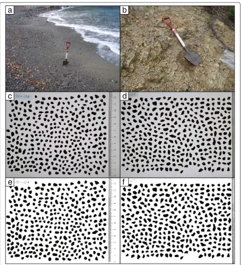
In this section, we apply our shape parameter to digital images of samples of sedimentary materials collected from modern beaches and slopes in the Masaki area of Eastern Japan (Figs. 9 and 10). The lithology of this region is mainly Cretaceous rhyolite, dacite, sandy siltstone, sandstone, and conglomerate (Shimazu et al. 1970). The beach deposits con-sist primarily of coarse-grained sands to granules with peb-bles, which are well-abraded by wave action on the beach (Fig. 10a). The slope deposits in this area comprise heavily weathered Cretaceous basement rocks, which occur as angu-lar granule- to pebble-sized clasts (Fig. 10b). Thus, the slope deposits can be considered immature clastics, while the beach deposits represent more mature clastic material. We selected these two types of materials for roundness analysis because they differ markedly in particle roundness, but both have a fairly coarse grain-size distribution.

Grain size distribution

A total of eight sedimentary samples were selected from beach and slope environments for this study, consisting of four beach deposits, referred to as B1, B2, B3, and B4, and four slope deposits, referred to as S1, S2, S3, and S4. Before shape analysis, their grain-size distributions were measured using a sieve ranging from −5.0 to 4.0 phi with 0.5 phi intervals (Fig. 11). Median grain sizes of the deposits in each environment were 0.33 (B1), −0.50 (B2),−1.25 (B3), and−0.50 (B4) phi for the beach deposits, and −3.18 (S1), −5.00 (S2), −4.77 (S3), and−2.47 (S4) phi for the slope deposits. The range between the first and third quartiles in the grain size distribution can be considered a proxy for the degree of sorting. Thus, these ranges in each environment were 0.821 to 0.869 (B1),−1.34 to 0.50 (B2),−1.93 to−0.40 (B3), and−1.70 to 0.16 (B4) phi

for the beach deposits and −3.96 to −1.96 (S1), −5.00 to −4.94 (S2), −5.00 to −4.30 (S3), and −3.46 to −1.33 (S4) phi for the slope deposits. Together, these data in-dicate that the beach deposits were finer than the slope deposits but had similar degree of sorting.

R distribution

The Rvalues were measured using ImageJ software, fol-lowing the above-described methodology. The measured Rdistributions in these two deposits are shown in Fig. 12. The median R of deposits in each environment was 0.847 (B1), 0.860 (B2), 0.865 (B3), and 0.866 (B4) for the beach deposits and 0.764 (S1), 0.778 (S2), 0.746 (S3), and 0.784 (S4) for the slope deposits. The range between the first and third quartiles of Rin the deposits of each environment were 0.821 to 0.869 (B1), 0.831 to 0.860 (B2), 0.835 to 0.889 (B3), and 0.838 to 0.889 (B4) for the beach deposits and 0.703 to 0.804 (S1), 0.759 to 0.792 (S2), 0.726 to 0.776 (S3), and 0.741 to 0.815 (S4) for the slope deposits. Together, these data indicate that the beach deposits were more rounded than the slope deposits.

Comparison between beach and slope deposits using R and grain-size distributions

Through the examination of bothRand grain-size distri-butions (Fig. 12), distinctive differences between beach and slope deposits are revealed. In order to compare the characteristics of the different deposits, a plot of the mean values and ranges between the first and third quartiles is shown for all samples in Fig. 12. This diagram shows clearly that the areas in which the beach deposits and slope deposits plot are completely separate. The beach de-posits had highRvalues and ranged from coarse-grained sands to granules. In contrast, the slope deposits had low R values and ranged in size from granules to pebbles. These distinct variations imply that there is a significant difference in cumulative energy between the two deposit types. The beach deposits comprise particles that are highly abraded by wave action and beach drift transport, whereas the slope deposits were comparatively unaffected by such physical abrasion. Therefore, the new roundness parameter Rcan be considered helpful for the study of sedimentary processes and the estimation of particle origins.

Conclusions

In this study, we propose a new particle roundness param-eter, R, which can be defined as the circularity cor-rected by the aspect ratio, and we demonstrate the calculation of this parameter from particle images, using ImageJ software. The results of this study can be summarized as follows:

1. The basic concept of the new roundness parameter

Rcan be defined as:

R¼Circularityþ Circularity_{perfect circle}−Circularity_{aspect ratio}

where Circularityperfect circle is the maximum value of circularity and Circularityaspect ratiois the circularity when only the aspect ratio varies from that of a perfect circle.

2. The effective diameter of a digital image suitable for

Rcalculations ranges from 100 to 1024 pixels, based

on shape analysis of test circle images of various sizes using ImageJ software.

3. The effective aspect ratio of digital images forR

calculations ranges from 10:1 to 10:10, based on shape analysis for various test circle and ellipse images in ImageJ software.

4. Given that a digital image is of an appropriate size,

circularity (CAR) is given by a sixth-degree polynomial

with respect to aspect ratio (ARI):

CAR¼0:826261þ0:337479ARI−0:335455ARI2

þ0:103642ARI3−0:0155562ARI4

þ0:00114582ARI5−0:0000330834ARI6

5. The new roundness parameterRis thus defined as:

R¼CIþð0:913−CARÞ

where CI is the circularity measured using ImageJ software.

6. Validation ofRusing the pebble images for visual

roundness provided by Krumbein (1941) reveals a

strong correlation coefficient (r= 0.937) between

Krumbein’s roundness andR.

7. Based on the application ofRto modern beach and

slope deposits, we can confirm that the new roundness

parameterRrepresents a useful new tool in the

analysis of particle shape.

Competing interests

The authors declare that they have no competing interests. Authors’contributions

YT originally produced the ideas forRand designed the study. YT and MI carried out the experimental study of modern sediment particles. All authors read and approved the final manuscript.

Acknowledgements

We thank the two anonymous reviewers who provided constructive comments and helpful suggestions. This research was partly supported by Grants-in-Aid for Scientific Research from the Japan Society for the Promotion of Science (Y. Takashimizu, no. 24740341). We also acknowledge Dr. A Urabe (Niigata University) who assisted us in sampling.

Author details

1_{Faculty of Education, Niigata University, Niigata 950-2181, Japan.}2_Oh-shima Elementary School, Joetsu 942-1103, Japan.

Received: 14 January 2015 Accepted: 27 December 2015

References

Abramoff MD, Magalhaes PJ, Ram SJ (2004) Image processing with ImageJ. Biophotonics Int 11:36_–42

Arasan S, Akbulut S, Hasiloglu S (2011) The relationship between the fractal dimension and shape properties of particle. J Civil Eng 15:1219–25. doi:10.1007/s12205-011-1310-x

Barrett PJ (1980) The shape of rock particles, a critical review. Sedimentology 27:291–303. doi:10.1111/j.1365-3091.1980.tb01179.x

Blott PJ, Pye K (2008) Particle shape: a review and new methods of characterization and classification. Sedimentology 55:31–63. doi:10.1111/j. 1365-3091.2007.00892.x

Bowman ET, Soga K, Drummond W (2001) Particle shape characterisation using Fourier descriptor analysis. Geotechnique 51:545–54

Clark MW (1981) Quantitative shape analysis: a review. Math Geol 13:303–20. doi:10.1007/BF01031516

Cox EP (1927) A method of assigning numerical and percentage values to the degree of roundness of sand grains. J Paleontol 1:179–83

Diepenbroek M, Bartholomä A, Ibbeken H (1992) How round is round? A new approach to the topic_‘roundness_’by Fourier grain shape analysis. Sedimentology 39:411–22. doi:10.1111/j.1365-3091.1992.tb02125.x Drevin RG (2007) Computational methods for the determination of roundness of

sedimentary particles. Math Geol 38:871–90. doi:10.1007/s11004-006-9051-y ImageJ user guide, 2012. ImageJ/Fiji 1.46, p. 187.

Itabashi K, Matsuo M, Naito M, Mori T (2004) Fractal analysis of visual chart of the particle shape and the comparison of shape parameters. Soils Found 44:143–56. doi:10.3208/sandf.44.143 (In Japanese)

Krumbein WC (1941) Measurement and geological significance of shape and roundness of sedimentary particles. J Sediment Petrol 11:64–72. doi:10.1306/ D42690F3-2B26-11D7-8648000102C1865D

Lees G (1963) A new method determining the angularity of particles. Sedimentology 3:2_–21. doi:10.1111/j.1365-3091.1964.tb00271.x Lira C, Pina P (2009) Automated grain shape measurements applied to beach

sands. J Coastal Res Spec Issue 56:1527–31

Orford JD, Whalley WB (1983) The use of the fractal dimension to quantify the morphology of irregular-shaped particles. Sedimentology 30:655_–68. doi:10.1111/j.1365-3091.1983.tb00700.x

Pettijohn FJ (1957) Sedimentary rocks, 2nd edn. Harper & Brothers, New York Powers MC (1953) A new roundness scale for sedimentary particles.

J Sediment Petrol 23:117_–9. doi:10.1306/D4269567-2B26-11D7-8648000102C1865D

Rittenhouse G (1943) A visual method of estimating two-dimensional sphericity. J Sediment Petrol 13:79–81

Roussillon T, Piegay H, Sivignon I, Tougne L, Lavigne F (2009) Automatic computation of pebble roundness using digital imagery and discrete geometry. Comput Geosci 35:1992–2000. doi:10.1016/j.cageo.2009.01.013 Schneider CA, Rasband WS, Eliceiri KW (2012) NIH Image to ImageJ: 25 years of

image analysis. Nat Methods 9:671_–5. doi:10.1038/nmeth.2089

Schwarcz HP, Shane KC (1969) Measurements of particle shape by Fourier analysis. Sedimentology 13:213–31. doi:10.1111/j.1365-3091.1969. tb00170.x

Shimazu M, Tanaka K, Yoshida T (1970) Geology of the Taro district. Quadrangle series, scale 1:50,000, Akita no. 18, Geol Surv Japan. 54 (In Japanese with English abstract).

Suzuki K, Sakai K, Ohta T (2013) Quantitative evaluation of grain shapes by utilizing Fourier and fractal analysis and implications for discriminating sedimentary environments. J Geol Soc Japan 119:205–16. doi:10.5575/geosoc. 2012.0085 (In Japanese with English abstract)

Suzuki K, Fujiwara H, Ohta T (2015) The evaluation of macroscopic and microscopic textures of sand grains using elliptic Fourier and principal component analysis: implications for the discrimination of sedimentary environments. Sedimentology 62:1184–97. doi:10.1111/sed.12183 Vallejo LE, Zhou Y (1995) The relationship between the fractal dimension

Wadell H (1932) Volume, shape, and roundness of rock particles. J Geol 40:443–51 Winkelmolen AM (1982) Critical remarks on grain parameters, with special emphasis

on shape. Sedimentology 29:255–65. doi:10.1111/j.1365-3091.1982.tb01722.x Yoshimura Y, Ogawa S (1993) A simple quantification method of grain shape of

granular materials such as sand. Doboku Gakkai Ronbunshu.J Japan Soc Civil Eng. No. 463/III-22:95_–103 (In Japanese with English abstract). doi: 10.2208/jscej. 1993.463_95

Submit your manuscript to a

journal and benefi t from:

7 Convenient online submission

7 Rigorous peer review

7 Immediate publication on acceptance

7 Open access: articles freely available online

7 High visibility within the fi eld

7 Retaining the copyright to your article