Greedy Feature Selection in Tree Kernel Spaces

(1)

International Doctorate School in Information and Communication Technologies

DISI - University of Trento

GREEDY FEATURE SELECTION IN

TREE KERNEL SPACES

Daniele Pighin

Advisor:

Prof. Marcello Federico

FBK, Human Language Technologies

Co-Advisor:

Prof. Alessandro Moschitti University of Trento, DISI

(2)

(3)

Abstract

Tree Kernel functions are powerful tools for solving different classes of problems requiring large amounts of structured information. Combined with accurate learning algorithms, such as Support Vector Machines, they allow us to directly encode rich syntactic data in our learning problems without requiring an explicit feature mapping function or deep specific domain knowledge.

However, as other very high dimensional kernel families, they come with two major drawbacks: first, the computational complexity induced by the dual representation makes them unpractical for very large datasets or for situations where very fast classifiers are necessary, e.g. real time systems or web applications; second, their implicit nature somehow limits their scientific appeal, as the implicit models that we learn cannot cast new light on the studied problems.

As a possible solution to these two problems, this Thesis presents an approach to feature selection for tree kernel functions in the context of Support Vector learning, based on a greedy exploration of the fragment space. Features are selected according to a gradient norm preservation criterion, i.e. we select the heaviest features that account for a large percentage of the gradient norm, and are explicitly modeled and represented. The result of the feature extraction process is a data structure that can be used todecode the input structured data, i.e. to explicitly describe a tree in terms of its more relevant fragments.

We present theoretical insights that justify the adopted strategy and detail the algorithms and data structures used to explore the feature space and store the most relevant features. Experiments on three different multi-class NLP tasks and data sets, namely question classification, relation extraction and semantic role labeling, confirm the theoretical findings and show that the decoding process can produce very fast and accurate linear classifiers, along with the explicit representation of the most relevant structured features identified for each class.

(4)

(5)

List of Algorithms

2.1 LEARN PERCEPTRON(T, D, alpha) . . . 15

4.1 FULL MINER(model) . . . 62

4.2 SIMPLE MINER(model, maxexp, maxdepth) . . . 65

4.3 BOUNDED MINER(model, maxexp, L) . . . 67

4.4 GREEDY MINER(model, L) . . . 70

4.5 ENCODE(frag, fragData, idxRoot) . . . 76

4.6 DECODE(tree, idxRoot) . . . 80

4.7 ENCODE STK(frag, fragData, idxRoot) . . . 84

(10)

(11)

List of Figures

2.1 Separating boundaries for a binary classification problem. . . 13

2.2 Maximum margin classification. . . 19

2.3 Kernel functions and linear separability . . . 22

2.4 Fragment space . . . 24

4.1 Architectural overview of an MLin classifier. . . 46

4.2 Architectural overview of an LOpt classifier. . . 47

4.3 Architectural overview of a Split classifier. . . 49

4.4 Recursive enumeration of the STK fragments encoded in a tree. . . 59

4.5 Recursive enumeration of the PTK fragments encoded in a tree. . . 61

4.6 Exemplification of a FragTree . . . 75

4.7 Examplification of an STKTree. . . 82

5.1 QC: included fragments vs. norm. . . 93

5.2 RE: percentage of norm retained after feature selection (1− ρ) vs. number of fragments. . . 94

5.3 SRL: percentage of norm retained after feature selection (1− ρ) vs. number of fragments. . . 95

(12)

lection . . . 97

5.6 SRL: Accuracy of the MLin model vs. norm after feature selection . . . 98

5.7 LOpt multiclass accuracy on the different tasks for different values of the threshold factor parameter L. . . 99

5.8 KSM and LSG time vs. number of mined fragments . . . 104

5.9 Average decoding time for trees of different size. . . 105

5.10 Classification efficiency of LOpt classifiers . . . 107

5.11 Learning time on the A1 class (SRL) with the Split configu-ration. . . 108

5.12 Learning efficiency of the Split architecture vs. STK on the A1 class. . . 109

(13)

List of Tables

5.1 Question classification dataset . . . 89

5.2 Relation extraction dataset . . . 89

5.3 Semantic role labeling dataset . . . 91

5.4 QC: F1-measure of STK vs. LOpt best model. . . 100

5.5 RE: F1-measure of STK vs. LOpt best model. . . 101

5.6 SRL: F1-measure of STK vs. LOpt best model. . . 102

A.1 QC: number of fragments mined for different values of the threshold factor parameter. . . 121

A.2 RE: number of fragments mined for different values of the threshold factor parameter. . . 122

A.3 SRL: number of fragments mined for different values of the threshold factor parameter. . . 122

A.4 Per-class best model parameters for the three tasks. . . 123

(14)

(15)

Chapter 1

Introduction

1.1 The Context

The last decades have seen a massive shift of attention from the so-called

knowledge based approaches to Natural Language Processing (NLP) in

favour ofcorpus based orstatistical approaches to the analysis of language.

In the former, linguists and domain experts would hard-code the rules and knowledge necessary to complete a task, wheras in the latter a system learns how to perform a task by means of rules inferred from text corpora in which the target phoenomena are instantiated. The research in Statistical NLP is indeed devoted to the development and exploitation of Machine Learning (ML) models and techniques for NLP applications.

(16)

In combination with SVMs, Kernel functions have been proven very useful to implicitly represent data in high dimensional spaces for NLP systems, e.g. [Kudo and Matsumoto, 2003, Cumby and Roth, 2003,Culotta and Sorensen, 2004, Toutanova et al., 2004, Shen et al., 2003, Kudo et al., 2005].

An especially interesting class of kernel functions for statistical NLP are

the so-called Tree Kernels (TK). A TK is a convolution kernel [Haussler,

1999] defined over pairs of trees. Convolution kernels are functions that

measure the similarity between structured object pairs in terms of the num-ber of substructures that they share. Each substructure is a feature in the convolution kernel space, and can be univocally associated with a compo-nent in a very-high dimensional space. The number and type of features is specific to each kernel function.

By using a TK, for example, it is possible to directly encode rich, struc-tured syntactic data into a learning problem without the need for manual feature design, as the kernel function will automatically evaluate the simi-larity between two parses as a measure of their overlap.

For all these reasons, the combination of a robust learning algorithm, such as Support Vector Machines, with the flexibility and ease of use of a tree kernel function is an effective and interesting way to explore new tasks and domains, where the knowledge about the relevant features can

be inadequate or insufficient, e.g. [Diab et al., 2008], or in those contexts

where a massive amount of syntactic information is needed, e.g. [Collins

and Duffy, 2002] and [Moschitti et al., 2008].

1.2 The Problem

Generality and implicitness, the key advantages of high dimensional ker-nels, are also the cause of their main drawbacks.

(17)

dimensional kernels very practical to deal with extremely large data sets (due to excessively long training time), or to cope with problems where classification speed is a must, e.g. when fast response times are required or large sets of unlabeled documents have to be classified. Concerning tree

kernels even the most efficient algorithms e.g. [Moschitti, 2006b, Zhang

et al., 2006], suffer from the burden imposed by the dual formulation of the problem, that makes them much less performant than conventional linear classifiers working in the primal space.

Concerning implicitness, high dimensional kernel spaces allow us to model very complex problems more easily and with smaller injections of domain knowledge, but on the other hand we cannot directly observe the most relevant features, which could provide useful insights towards a deeper understanding of the studied problems. In this respect, it is undeniable that corpus based approaches and especially kernel methods are not as

informa-tive as knowledge based methods when trying to explain why some model

performs better than others. Exploring the feature space of tree kernel func-tions, that can cope with large amounts of rich syntactic data, would indeed be a very promising way to discover new, relevant structured features.

Complexity and implicitness make the adoption of tree kernels less at-tractive for a number of possible users, like those who would be interested in performant solutions for real-world tasks and applications, such as in-dustries and IT companies, or those that would prefer approaches that can advance our understanding of linguistic processes, such as linguists, cog-nitivists or anyone interested in improving available models by means of error analysis and feature inspection.

Complexity-wise, feature selection techniques can offer a solution in many important cases. Still, even though very effective models exist for

kernel families defined over RN, such as polynomial or gaussian kernels

(18)

approaches that focus on, or can cope with, the rich space generated by a

convolution kernel are few and isolated [Kudo and Matsumoto, 2003,Suzuki

and Isozaki, 2005]. As for the implicitness of the result, to our knowledge there are no previous works that directly try to address this problem for high dimensional kernels.

1.3 Proposed solution

This thesis describes a methodology to employ feature selection in a very high dimensional kernel space as a possible solution to both problems. In particular, it will focus on the kernel space generated by TK functions in the context of a Support Vector Machine (SVM) learning framework.

The SVM optimizer is an effective device to select the most relevant examples (the support vectors) and to obtain a feature selection side-effect. Indeed, the weights expressed by the gradient of the SVM’s separating hyperplane implicitly establish a ranking between features in the kernel space. This property has been exploited in feature selection models based

on approximations or transformations of the gradient, e.g. [Rakotomamonjy,

2003], [Weston et al., 2003], [Guyon et al., 2002] or [Kudo and Matsumoto, 2003].

Tree kernels generate a huge feature space, in which each distinct tree sub-structure is mapped onto a different dimension. In this situation it is impossible to enumerate and rank all the features in the space. The only possibility is to start generating features in order of relevance, starting from the most relevant, and define a criterion to terminate the exploration.

(19)

still retain a large fraction of the gradient norm. As a consequence, we also preserve a large fraction of the margin of the original model, and therefore its accuracy. The relevant fragments are explicitly represented and stored

in a convenient data structure that we can then use to decode the data

of the original problem. We call decoding the process by which the input trees are projected onto an explicit, lower-dimensional space where each component accounts for the presence of a relevant feature. The decoded data can then be used to carry out fast learning and classification in the projected space.

The data structure that we use to store the relevant fragment can actually be considered as a graphical representation of a set of explicit algorithms to extract structured features from the input data. In this respect, the ex-pressivity of the rules that we can induce is only limited by the exex-pressivity of the target kernel space, and the kind of rules that can be produced is a combination of the structured input data and the characteristics of the kernel. This kind of representation allows us to actually unleash all the potential for automatic feature discovery of tree kernels, generating and weighing relevant features in the huge fragment space. We select the most relevant structured features and encode them as linear attributes in a tra-ditional attribute-value representation, thus combining the advantages of both representations.

The suggested line of research poses modeling and computational chal-lenges, collocating itself in the largely unexplored research field of feature selection for convolution kernels and in an area of interest between:

• machine learning, since the feature selection technique moves from

(20)

• data mining, since the algorithms and the data structure that we

em-ploy are heavily influenced by previous work in this field, e.g. [Zaki,

2002, Pei et al., 2001];

• computational linguistics, since by proposing an approach that can

make (part of) the tree kernel space explicit we hope to offer the community a valuable technique for discovering and engineering new structured features for a wide class of problems.

A note on related publications.

Parts of this work have already been peer-reviwed by the scientific community. In [Pighin and Moschitti, 2009a], we presented an earlier version of our feature selec-tion framework based on the SIMLE MINER(·) algorithm (discussed in Sec. 4.5.2), and applied it to a semantic role labeling benchmark. In that context, we also considered the very demanding task of boundary classification for semantic role labeling, includ-ing 1,000,000 traininclud-ing instances. We showed that the LOpt (Sec. 4.1.2) and Split (Sec. 4.1.3) architectures can result in very accurate and fast learning and classification cycles.

In [Pighin and Moschitti, 2009b], we mostly focused on the explicit representation of the tree kernel feature space, by tackling the question classification task with the LOpt architecture (4.1.2) and the BOUNDED MINER(·) algorithm (Sec. 4.5.3). We demonstrated that feature selection in the TK space is a very effective way to automatically engineer relevant structured features.

The theoretical framework, outlined in Section4.3, and the latest version of the mining algorithm, GREEDY MINER(·) (Sec. 4.5.4), are currently under review.

1.4 Innovative Aspects

The thesis presents the following main points of novelty:

(21)

margin and therefore on the error rate of the classifier (Lemma 4.3.1). We show how the peculiarities of the TK space make it possible to discard an exponentially large number of features while preserving most of the gradient

norm (Lemma 4.3.4). The combination of these two findings establishes the

basis of our feature selection technique. To our best knowledge, this is the first attempt to feature selection in TK spaces that clearly establishes a link between the empirical model and the theory, thus providing a solid starting point for the exploration of the feature space of other structural kernel families.

Insights about the inner working of TK functions. Due to TK functions implicit

formulation, the nature of the feature space they generate and the behaviour of individual features in these spaces is by and large obscure. We clearly break down the process by which TK functions generate their rich feature space, and provide insights about the kind of information that different

kernel functions can represent (Sec. 4.4).

A greedy strategy to mine the TK feature space. We describe an algorithm for the

exploration of the TK space (Alg. 4.4) that can efficiently select the most

relevant features in the high dimensional tree kernel space. Supported by our theoretical claims, the algorithm can implement a very aggressive selection strategy. The gradient norm in the TK space is employed to guide the selection process and to estimate the relevance of individual fragments. The space is explored in a small-to-large fashion, as according to the kernel definition smaller fragments have more chances of being highly relevant (Sec. 4.5).

Efficient data structure and algorithms for fragment indexing. We introduce a data

(22)

frag-ments, and design algorithms for fragment indexing and matching that have linear complexity with respect to the number of nodes of the input trees

(Sec. 4.6).

An explicit representation of the fragment space. Our data structures store

plicit representations of the most relevant fragments. This allows us to ex-ploit the feature-discovery capabilities of tree kernel functions in very fast linear classifiers, by projecting the input data onto a lower dimensional space where only the most relevant fragments are accounted for. The frag-ments that we isolate can be a valuable tool in the hands of linguists and domain experts to gain insights on the problems at study.

Three architectures for exploiting feature selection in TK spaces. We present three

different architectures that stress different aspects of the feature selection

methodology (Sec. 4.1): the link with the theoretical framework (MLin,

Sec. 4.1.1), classification accuracy (LOpt, Sec. 4.1.2) and training time

effi-ciency (Split, Sec.4.1.3).

A general framework for feature selection in high dimensional spaces. Even though

we focus on a specific class of kernel functions, the framework that we introduce is general enough to be easily extended to include other families of kernel functions.

1.5 Structure of the Thesis

The rest of the document is structured as follows.

Chapter2introduces notations and concepts that will be used throughout

the discussion, namely support vector machines, kernel functions, tree

(23)

relevant results in the previous work concerning the use of tree kernels for

NLP and feature selection techniques for kernel learning. Chapter4details

the solution that we advocate, in terms of theoretical insights, algorithms

and data structures. Chapter 5 presents the setup and the results of an

extensive empirical evaluation on three very different benchmarks: ques-tion classificaques-tion, relaques-tion extracques-tion and semantic role labeling. Finally,

Chapter 6 draws the conclusions and hints possible directions for future

(24)

(25)

Chapter 2

Preliminary Concepts

In this chapter, we introduce terminology and concepts that will be used throughout the rest of the discussion. The chapter is structured as follows:

Section2.1 explains the problem of classification and introduces linear

clas-sifiers; Section2.1.1 describes maximum margin classifiers and support

vec-tor machines; Section 2.1.3 shows how the kernel trick can allow a linear

classifier to cope with non linearly separable problems; Section2.2 explains

tree kernel functions in more detail, and presents a selection of relevant TK

families; finally, Section 2.3 outlines the basic concepts behind feature

se-lection.

2.1 Linear Classifiers

The problem of classification consists of learning how to partition elements

of some set O into a finite number of classes C. As an example, we may

want to assign the most appropriate topical label to some news (e.g. politics, economics, sports or technology), or, given a collection of X-rays lung scans, we may be interested in recognizing the cases showing evidence of tumoral

forms. If the problem only involves two classes, i.e. |C| = 2, the classifier is

called a binary classifier. If |C| > 2, then it is referred to as a multi-class

(26)

Classification is very conveniently handled as a supervised learning

problem, where a learning algorithm learns an approximation g of the

func-tion f : O → C that assigns the proper class to any object o ∈ O, based on

the observations provided by a training set T ⊂ O × C, in which training

points oi ∈ O are paired with their correct label f(oi) ∈ C. Learning is

a generalization process, since the learner must be capable of abstracting from individual traits of the training data in order to be able to cope with

examples never seen before, i.e. the test data E ⊂ O. Here, an important

assumption is that the examples that make up the training and test data are independent and identically distributed (iid), meaning that they are sampled from a fixed, yet possibly unkown, distribution independently from each other.

For complex objects, a mapping function φ : O → RN can provide a

so-called feature based representation of the objects oi ∈ O as vectors

xi ∈ RN, where the scalar product can be used as a measure of pairwise

similarity. In this case, learning a classifier requires to estimate a function

g : RN →R that can separate the examples belonging to different classes.

The mapping function φ(·) summarizes the process of feature design, a

rel-evant aspect of classifier design that requires efforts, expertise and domain knowledge in order to find a convenient representation for the (potentially

complex and structured) objects of O in RN.

Given a set of training points T, it is generally possible to find more

than one function that can separate them. Figure 2.1 gives a graphical

(27)

Figure 2.1: Separating boundaries for a binary classification problem.

Remp(g) = 1_|T| |T|

X

i=1

1

2|f(xi)− g(xi)| ,

but it does not give us information about the risk, i.e. the error on the test data, and therefore it is not a useful tool for comparing different choices of

g.

Intuitively, we can imagine that very complex functions would be better at outlining the boundaries of class distributions. On the other hand, such carefully tailored boundaries would increase the risk of over-fitting the training data, i.e. of learning a classifier which performs very well on the training data but not as well on a training sample having a distribution even slightly different.

Statistical learning theory [Vapnik, 1998] (SLT) uses the the

Vapnik-Chervonenkis (VC) dimension of a class of functions F as a measure of

the trade-off between its capacity to separate a set of data points and

(28)

maximum number of points that can be shattered by F. F is said to shatter

a set of points P iff, ∀P1, P2 ⊂ P | P1⊕P2 = P, 1 ∃f ∈ F so that P1 and P2

are separated by f, i.e. if there is at least one function in the family that

can be used to define a boundary between any partition of the points. A collection of related results shows that it is very important to consider classes of functions that have just enough capacity to separate the training

points [Sch¨olkopf and Smola, 2001]. Interestingly enough, knowing the VC

dimension of a decision function also allows us to estimate an upper bound on the risk of the classifier, i.e. the error on any possible selection of test

points, as explained by the following theorem [Vapnik, 1998]:

Theorem 2.1.1. Let h be the VC dimension of a class of functions F. Then, with probability 1− δ, the risk R(f) of a classifier f ∈ F on a test set of ` examples is bounded by:

R(g) = Remp(g) +

s

h(log2`

h + 1)− logδ4

` . (2.1)

The structural risk minimization (SRM) principle is a straightforward consequence of these results: when designing a classifier, the decision function should be selected so as to

• minimize the empirical risk, and

• belong to a family with the lowest possible VC dimension.

If we can satisfy these two properties, we minimize Equation2.1 and identify

the function(s) with the lowest bound on the test error.

Linear functions, which have a low VC dimension, are hence interesting candidates for the definition of the boundary if the training data are linearly separable.

(29)

Algorithm 2.1 LEARN PERCEPTRON(T, D, alpha)

main

b ←0,w ←0N

ford ∈ {1, . . . , D}

do

      

for each hyi,xii ∈ T

do

  

∆ =α(yi−sgn(w ·xi+b))

w ←w + ∆xi

b ← b+ ∆

The decision function of a linear classifier is a hyperplane in RN, i.e.:

g(x) = sgn(w ·x +b), (2.2)

where x is a point to classify and w and b are called the gradient and the

bias of the hyperplane, respectively. A set of points x1, . . . , x` are linearly

separable if ∃γ ∈ R+,w ∈ RN, b ∈ R so that ∀i = 1, . . . , `, it holds that

yi(w ·xi+b)≥ γ. Here, yi ∈Ris the label associated to the point xi, that

marks it as belonging (or not) to the target class. The minimum distance

between two points in different classes along the direction of w, γ, is called

the margin of the classifier.

Different learners use different algorithms to estimate the weight vector

w and the bias b, generally resulting in different boundaries for the same

data and, as a consequence, in different margins. A very simple algorithm for

learning a linear classifier is the perceptron [Rosenblatt, 1958]. The learning

process consists of one or more iterations over the training points. Whenever the perceptron misclassifies an example, the components of the gradient

are updated accordingly. The learning algorithm is shown in Algorithm 2.1,

where:

T = S`_i₌₁hyi,xii is the training set, yi ∈ {0,1},

0< α ≤ 1 is the learning rate of the perceptron, and

(30)

2.1.1 Maximum Margin and Support Vector Machines

Among the class of linear functions, an especially interesting family is that of maximum margin hyperplanes, i.e. the hyperplanes that are maximally distant from the examples of the two training classes. As we have seen

before, this property is expressed by the marginγ of the hyperplane. Indeed,

statistical learning theory shows that maximum margin hyperplanes have a lower VC dimension than other hyperplanes. As a consequence, they show better generalization performance than any other linear functions.

As shown by the following theorem, the margin of the hyperplane is in

fact inversely proportional to the bound on the risk [Bartlett and

Shawe-Taylor, 1998]:

Theorem 2.1.2. Let

C = {x →w ·x :kwk ≤ 1, kxk ≤ R}

be the class of real-valued functions defined in a ball of radius R in RN.

Then there is a constant k such that for any classifier h = sgn(c) ∈sgn(C), for any sample of ` randomly selected examples, if all the ` examples are separated with margin γ, i.e. |w ·x| ≥ γ, then with probability 1− δ the error over the sample is bounded by

k `

_R₂

γ2log2` + log1_δ

.

Furthermore, if b examples are separated with margin less than γ, then with probability 1− δ the error on the ` examples is less than

b ` +

s

k `

_R₂

γ2log2` + log1_δ

.

(31)

ma-chine that implements the structural risk minimization principle by forc-ing margin maximization when learnforc-ing a linear solution to a classification task 2_.

Given a set of training examples T = {hx1, y1i, . . . , hx`, y`i}, with yi ∈

{+1, −1}, the optimization problem solved by the SVM optimizer is

Maximize: 12kwk2

Subject to: yi(w ·xi − b)≥ 1 ∀i = 1, . . . , ` , (2.3)

where the space is implicitly normalized so that the closest points are at distance 1 from the hyperplane. This is generally referred to as the primal optimization problem.

By introducting Lagrange multipliers αi ≥0, the previous conditions can

be rewritten as the Lagrangian:

L(w, b,α_{) = 12}kwk2 ₋X`

i=1

αi(yi(w ·xi − b)−1) (2.4)

where w and b are the primal variables, while α is the dual variable.

Solving the problem requires to find a saddle point of the Lagrangian,

by minimizing L for the primal variables and maximizing it for the dual

variables. By deriving for w and b we obtain that

(32)

w∗ ₌X` i=1

αiyixi (2.5)

`

X

i=1

αiyi = 0 . (2.6)

If we substitute 2.5 and 2.6 in 2.4 we can derive the dual form of the

optimization problem, where the only variable is the dual variable α:

Maximize: W(α) = X`

i=1

αi − 1₂X i,j

αiαjyiyjxi ·xj (2.7)

Subject to: X`

i=1

αiyi = 0 , αi ≥ 0.

Practically, only a few αi will be greater than zero. The corresponding

xi are called the support vectors of the decision function, and lie exactly on

the margin, i.e. they satisfy yi(w ·xi+b) = 1.

Figure2.2shows a simple two dimensional classification problem and the

maximum margin hyperplane that separates the two classes. The gradientw

is normal to the separating hyperplane, and the margin measures γ = 2

kwk.

The bias b is the distance, along the direction of w, of the hyperplane from

the origin.

2.1.2 Soft-margin SVMs

(33)

wx+

b=1

wx+

b=0

wx+

b=−

1

γ₌

2 kwk

b

w

Figure 2.2: Maximum margin classification. side of the hypothetical boundary.

Soft margin SVMs [Cortes and Vapnik, 1995] extend the range of

appli-cability of SVMs by learning a hyperplane that allows for some examples within the margin, while still trying to maximize inter-class distance. This result is obtained by including in the optimization problem slack variables

ξi that allow a training point xi to fall also within the margin, i.e.:

Maximize: 12kwk2 ₊_CX`

i=1

ξ_i

Subject to: yi(w ·xi − b)≥ 1− ξi

0 ≤ αi ≤ C ,

where the costant C > 0 accounts for the trade-off between classification

errors, i.e. examples within the margin, and margin maximization.

(34)

soft margin SVM fall under the category of quadratic problems (QP), for

which very efficient solvers exist [Nocedal and Wright, 2000].

2.1.3 Kernel Machines

By combining together i) the optimization of QP, ii) the low VC dimension of the large margin classifier, and iii) the ability to cope with mislabeled data, thanks to the soft margin formulation, an SVM is an efficient, accurate and robust solution which is very attractive for learning linear classification

problems. By applying the so-called kernel trick [Aizerman et al., 1964],

as explained below, these interesting features can be exploited also to tackle classification problems that require a more complex boundary to be separated.

If we substitute (2.5) in (2.2), we obtain the decision function of the SVM

for a test point x, i.e.:

g(x) = sgn (w ·x +b)

= sgn

_X_`

i=1

αiyixi

!

x +b

!

= sgn

_X_`

i=1

αiyixi·x

!

+b

!

, (2.8)

and we can observe that the result only depends on the dot product between pairs of points rather than on the individual points. Similarly, also the

optimization problem in 2.7 depends on the dot product.

Since both training and classification do not depend on individual test points, the inner product in all the equations can be replaced with a function

(35)

objects O we can define a function k : O × O → H so that:

k(oi, oj) = φ(oi)· φ(oj) = xi ·xj , xi,xj ∈ HN , (2.9)

i.e. a function that evaluates the inner product in some high-dimensional

space HN _{by representing the input objects} _o_i_{, o}_j _{∈ O} _{via a mapping}

function φ :O → HN_{, where} _H ₌

R or H =C.

As an example, let us consider the polynomial kernel of degree d, which

is defined as

K(a,b) = (a·b+ 1)d _. _(2.10)

If d = 2 and a,b ∈ R2, then we can write (2.10) explicitly as:

K(a,b) =(a1b1 +a2b2 + 1)2

=a2

1b21 +a22b22 + 1 + 2a1b1 + 2a2b2 + 2a1b1a2b2

=[a2

1, a22,1,

√

2a1a2,√2a1,√2a2]·[b21, b22,1,

√

2b1b2,√2b1,√2b2]

=φ(a)· φ(b), (2.11)

and observe that the φ(·) maps a vector onto a space where also all the

conjunctions of features having length up to d are represented, i.e. a1a2

and b1b2.

Using the kernel trick, i.e. replacing dot products with a kernel function, we can rewrite the decision function of the SVM as:

c(o) = sgn X`

i=1

αiyik(oi, o) +b

!

. (2.12)

If the mapping is appropriate, we can expect our objects to be mapped onto a space with enough dimensions to make the problem linearly separable. As

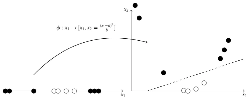
an example, consider the set of points in Figure 2.3, which are not linearly

(36)

x1

x2

x1

φ:x1→[x1, x2= (x1−a)_b 2]

Figure 2.3: Kernel functions and linear separability - The points are not linearly sep-arable in the original 1-dimensional space (left), but they are sepsep-arable in the higher dimensional space induced by the mapping φ(·) (right).

by a kernel function, we can represent them in a higher dimensional space where a linear separation is possible.

The condition to apply the kernel trick is that k must be equivalent

to a dot product in some high dimensional space. According to Mercer’s

theorem [Mercer, 1909], for real valued functions the equivalence holds if k

is continuous, symmetric and positive semidefinite, but other theorems can be used to demonstrate that a function is a valid kernel also in different

cases [Sch¨olkopf and Smola, 2001].

As a side effect of these conditions, if c > 0 and k1, k2 : O × O → H

are valid kernel functions, then in all the following cases k is a valid kernel

too:

k(oi, oj) = ck1(oi, oj)

k(oi, oj) = c+k1(oi, oj)

k(oi, oj) = k1(oi, oj) +k2(oi, oj)

k(oi, oj) = k1(oi, oj)· k2(oi, oj)

(37)

corresponding mapping φk(·) to be explicit, as it suffices to demonstrate

that such mapping exists by satisfying Mercer’s theorem or equivalent con-ditions. This allows us to evaluate pairwise similarity in very high dimen-sional spaces using very compact and implicit definitions.

It should be noted that the kernel trick is not a peculiarity of support vector learning, as it can be applied to any learning algorithm for which both the training and the decision function can be expressed in terms of dot products. Learning algorithms that can be reformulated to exploit the kernel trick are generally referred to as kernel machines. For example, also the perceptron algorithm can be rewritten in terms of dot products, which

can then be replaced by a kernel function [Freund and Schapire, 1999].

2.2 Tree Kernel Functions

For the scope of this thesis, we focus on a specific class of kernel functions that can directly estimate pairwise similarity between trees, the so-called Tree Kernel (TK) functions. Before describing TKs in more detail, it is con-venient to introduce notation and terminology that will be used throughout the rest of the discussion.

Formally, a tree is a simple, connected and undirected graph. As such,

a tree t is defined by the a pair hNt, Eti, where Nt is the set of vertices, or

nodes, of t, and Et the set of edges. A tree is rooted if one node has been

designated as the root, in which case the edges have a natural orientation, towards or away from the root. In a rooted tree, the parent of a node is the node connected to it on the path to the root; every node except the root

has a unique parent. A child of a node v is a node of which v is parent. A

(38)

A

B A

A

B A

A

B A

C

A

B A

C A

C

D

B A

D

B A

C

1 2 3 4 5 6 7

t1 A

B A

C

t2 D

B A

C

φ(t1) = [2,1,1,1,1,0,0]

φ(t2) = [0,0,0,0,1,1,1] K(t1, t2) =hφ(t1), φ(t2)i= 1

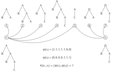
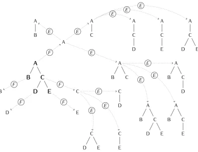
Figure 2.4: Fragment space- The fragment space generated by two trees, and the resulting kernel product as evaluated by a tree kernel function.

is specified for the children of each node. In the rest of the discussion, the

word tree will always be used to refer to a rooted and ordered tree.

A tree kernel is a convolution kernel [Haussler, 1999] defined over tree

pairs, i.e. a kernel that evaluates the similarity between two trees by estimating the degree of their overlap. The overlap is estimated by counting the number of substructures, or fragments shared between the two trees. It

does so by establishing an implicit mapping φ(·) that associates different

fragments with different dimensions in a high-dimensional space.

Basically, each tree t is mapped onto a vector x = [x(1)_{, . . . , x}(N)_{], whose}

attributes x(i) _{account for the occurrences within} _t _{of the fragment} _f_i_{, i.e.}

the fragment mapped onto the ith _{dimension of the} _N_{-dimensional kernel}

space, and the kernel product is equivalent to the scalar product between

pairs of such vectors, as exemplified in Figure 2.4. Here, the tree labeled

(39)

the right, t2, contains the fragments labeled 5-7. Since the two trees only

share the fragment labeled 5, the kernel product evaluates to 1.

Actually, each fragment can also be weighted according to one or more decay factors that penalize larger substructures. Decay factors are intro-duced to compensate for the intrinsic dependence between a large fragment and the smaller fragments it contains. For example, if we consider the

frag-ment labeled as 4 in Figure 2.4 we can observe that it is a super-structure

of fragments 1, 2, 3 and 5, which are already accounted for. In turn, fragment 3 can be expressed as a combination of 1 and 5.

Different kernel functions (e.g. [Collins and Duffy, 2002, Kashima and

Koyanagi, 2002,Viswanathan and Smola, 2003, Moschitti, 2006b]) result in different constraints to the construction of fragments, that affect the topology and number of substructures that can be observed in a tree. More precisely, each kernel function defines implicitly: i) constraints about the topology of admissible fragments; ii) rules to generate the fragments encoded in a tree; iii) weights to be assigned to each fragment depending on how it is generated. All these aspects will be explained in more detail in the next sections and chapters.

The rest of this section details two kernel families that are especially interesting for computational linguistics, as they can effectively model

prob-lems involving constituency and dependency parsed data. In Section 3.1,

other tree kernels and their applications to natural language processing will be discussed.

2.2.1 The Syntactic Tree Kernel

The Syntactic Tree Kernel (STK) [Collins and Duffy, 2001, Collins and

(40)

for tasks involving constituency parsed texts as it allows to directly employ rich syntactic data in the learning algorithm.

LetF = {f1, f2, . . . , f|F|}be an explicit representation of all the fragments

encoded by the training data, i.e. its fragment space. Let χi(n) be an

indicator function3_{, equal to 1 if the target fragment} _f_i _{is rooted at node} _n_,

and equal to 0 otherwise. The STK function over t1 and t2 is defined as

STK(t1, t2) = X

n1∈N1

X

n2∈N2

∆(n1, n2), (2.13)

where N1 and N2 are the sets of nodes in t1 and t2, respectively and

∆(n1, n2) =

|F|

X

i=1

χi(n1)χi(n2). (2.14)

The ∆ function counts the number of subtrees rooted in n1 and n2 and

can be evaluated as:

1. if the productions at n1 and n2 are different, then ∆(n1, n2) = 0;

2. if the productions at n1 and n2 are the same, and n1 and n2 have only

leaf children (they are pre-terminal symbols), then ∆(n1, n2) =λ;

3. if the productions at n1 and n2 are the same, and n1 and n2 are not

pre-terminals then

∆(n1, n2) = λ

lY(cn₁)

j=1

(1 + ∆(cj

n1, cjn2)), (2.15)

(41)

where l(cn1) is the number of children of n1, cjn is the j-th child of node n,

and λ is a decay factor penalizing larger structures.

2.2.2 The Partial Tree Kernel

The Partial Tree Kernel (PTK) [Moschitti, 2006a] defines a more general

class of fragments, allowing any connected substructure of a tree to be considered as a valid fragment. Unlike the STK, it does not require that two nodes have the same productions in order to contribute to the kernel product. This feature makes it more appropriate to deal, for example, with dependency parsed text.

The evaluation of the common fragments rooted in two nodes n1 and n2

involves the evaluation of all the possible subsequences of the children of both nodes, and considers all the identical subsequences. As an example,

letn1 = (S(DT)(JJ)(N)) andn2 = (S(DT)(N)). Even though the productions

of the two nodes are different, we can observe that there is one children

sequence of length 2 that is shared across n1 and n2, i.e. [DT, NN]. As a

consequence, the two nodes also share two children sequences of length 1,

i.e. [DT] and [NN]. This process is no different than applying a sequence

kernel [Lodhi et al., 2002] to the nodes children.

More formally, let Zi be an index sequence associated with the ordered

child sequence ci of the node ni. Let Zi[k] be the k-th element of Z, and

Zi[−1] a notation for its last element. For example, if n = (A(B)(C)(D)), two

of its possible index sequences would be Z = [0,2] (selecting nodes B and

D) or Z = [2] (selecting node D).

Let l(Zi) be the length of Zi. Zimilarly to the STK, the PTK can be

evaluated as:

PTK(t1, t2) = X

n1∈N1

X

n2∈N2

(42)

but in this case the ∆ function is defined as:

∆(n1, n2) = µ



_λ2 ₊ X

Z1,Z2|l(Z1)=l(Z2)

λd(Z1)+d(Z2)

lY(Z1)

i=1

∆(cZ1[i]

1 , cZ22[i])



 _(2.17)

where

d(Zi) =

(

1 , if l(Zi) = 0

Zi[−1]− Zi[1] + 1 , else. (2.18)

accounts for the length of the sequence Zi in terms of the difference between

the last and the first element in the sequence, plus 1. Thus, for example:

d([2,3,4,5]) = d([2,5]) =d([2,4,5]) = 5−2 + 1 = 4 ,

and

d([2]) = 2−2 + 1 = 1 .

The PTK makes use of two decay factors: µ, which accounts for the

depth of the fragment, and λ, which accounts for the number of nodes in the

fragment.

(43)

2.2.3 Tree Kernel Normalization

The output of tree kernel functions is generally normalized in the interval

[0,1]. Since the norm of a tree t can be evaluated as:

ktkTK = pφ(t)· φ(t) = pTK(t, t) , (2.19)

where φ(·) is the explicit mapping of a generic kernel function TK, to

nor-malize TK(ti, tj) it is sufficient to replace it with:

f

TK(ti, tj) = TK

_t

i

ktik,

tj

ktjk

= TK(_kt ti, tj)

ik · ktjk

= p φ(ti) TK(ti, ti) ·

φ(tj)

p

TK(tj, tj)

= p φ(ti)

φ(ti)· φ(ti) ·

φ(tj)

p

φ(tj)· φ(tj) . (2.20)

2.3 Feature Selection Techniques

The problem of variable, or feature, selection arises in almost any research field, from gene microarray data analysis to image recognition and text categorization, where common machine learning problems are characterized by the necessity to cope with very large data sets, typically described by high-dimensional vectors in some dot product space.

Feature selection is the name given to a set of techniques commonly used to improve the quality of the models learned with machine learning methods. Depending on the context, it can aim to alleviate the effect of

the curse of dimensionality [Bellman, 1961], enhance the generalization

(44)

process or make the models more easily interpretable. A very interesting

and comprehensive survey on feature selection is carried out in [Guyon and

Elisseeff, 2003].

As explained in Section 2.1.3, when using kernel functions we generally

do not know explicitly all (if any) of the attributes that will represent the

objects in the kernel space. Instead, a mapping function φ(·) projects an

example in some implicit feature space, generally very high if not infinite-dimensional. Given the very high dimensionality of kernel spaces, feature selection is a critical task for the realization of compact, accurate and ef-ficient predictors. Feature selection strategies are typically divided into three main categories:

filters, where features are selected independently of the learning algorithm. Features are filtered based on some measure suggested by the data, such as the correlation between features and labels (e.g. mutual in-formation);

wrappers, in which the learning algorithm is used as a black box to search the space of feature subsets. The learning machine is trained on dif-ferent subsets of features. Then, the accuracy of the resulting model is evaluated and used to focus the search;

embedded methods, that incorporate the search of the feature subsets into the optimization problem of the learning algorithm. A common strategy is to minimize the cost function of the learner while enforcing some constraints on the dimensionality of the input space.

Filter methods are very generic, yet the kind of induction used by the filter may be utterly different from the one employed by the learning machine and introduce a new source of bias in the learning process.

(45)

of features and the learning, and no further bias is introduced. On the other hand, wrappers are computationally very expensive, and for very large feature spaces only rough searches (generally involving greedy algorithms) can realistically be performed.

Embedded methods share the virtues of wrapper methods, with the fur-ther advantage that the optimization problem can be refined in many subtle ways. The main disadvantages of this approach are the complexity of the implementation and the general impossibility to decouple the feature se-lection model from the embedding learning machine.

In Section 3.2 we will discuss a selection of interesting feature selection

(46)

(47)

Chapter 3

Related Work

This chapter presents a selection of relevant work concerning the tree nels and feature selection approaches for support vector machines and ker-nel methods.

In particular, in Section 3.1, we will focus our attention on several

in-teresting applications of TKs that show how they have been successfully applied to a wide range of different tasks. These applications demonstrate the flexibility of the tool and its importance as a solution for all those situ-ations where the clues about the relevant features are not enough to define accurate explicit models. These works motivate the interest towards effec-tive feature selection strategies, and especially towards ways of making the most relevant fragments observable.

Concerning feature selection, in Section 3.2 we present an overview of

(48)

3.1 Tree Kernels for Natural Language Processing

Seminal works for TK learning are [Collins and Duffy, 2001, Collins and

Duffy, 2002], where the authors define the STK (see Section 2.2.1) and apply it to the task of parse reranking, in conjunction with the voted perceptron

algorithm of [Freund and Schapire, 1999]. They also define a variant of

the algorithm, the Tagging Kernel, employed for labeling tasks where a

sentence S can be described as a sequence of states S = [n1, n2, . . . , n|s|,

with each state ni being a pair hwi, hii. Here, wi is the i-th word in the

sentence and hi the associated tag. The tagging kernel, defined over pairs

of state sequences, is equivalent to the evaluation of the STK on trees

where each state ni is a node whose children are hi, wi and the next state

in the sequence ni+1, e.g.

n1

h1 w1 n2

h2 w2 .. . .

This is an interesting example of the flexibility of tree kernels, that due to their generality can be used to abstract a wide range of more specific problems and to prototype effective working solutions.

The PTK is introduced in [Moschitti, 2006a], where it is applied to the

(49)

in accuracy of the PTK can mostly be ascribed to the extra fragments generated by the PTK, possibly overfitting the training data, and to the dimensionality of the fragment space.

In [Moschitti et al., 2007], the PTK is employed to build a tree-kernel driven model for question answering. Sequences (with gaps) of words or

POS tags, which could be modeled using string kernels [Lodhi et al., 2002,

Cancedda et al., 2003], are here evaluated by a PTK on pairs of ad-hoc engineered trees. A fake syntax is used as a container for the sequences of words/POS tags, and to allow the computation of the tree kernel.

In [Zhang and Lee, 2003], the authors describe a variant of the STK that also assigns a weight to terminal nodes, whereas the STK would not consider them independently of their pre-terminal parents. This allows the kernel to fall back to a bag of words (BOW) model in the cases where there is no syntactic overlap between two trees, i.e. the only contribution comes from the leaves. They also introduce a second decay factor that accounts for the depth of the trees, similarly to the PTK. The resulting kernel is applied to the task of coarse grained question classification.

(50)

In [Diab et al., 2008], TKs are used to tackle the problem of semantic role labeling for Arabic. Unlike the English language, where a set of rel-evant lexical and syntactic features for the task have been identified and

commonly exploited [Gildea and Jurafsky, 2002, Pradhan et al., 2005, Xue

and Palmer, 2004], this kind of linguistic knowledge is not available for the Arabic language. The STK is therefore used to automatically discover relevant features by only relying on the information encoded in parse trees. The results show that TKs are valuable tools for tackling in an effective way tasks where there is not enough knowledge to explicitly design a set of relevant features, but there is high availability of rich syntactic data.

[Kazama and Torisawa, 2005] describe an interesting algorithm to speed up TK evaluation. This algorithm looks for node pairs in which the rooted-subtrees share many substructures (malicious nodes) and applies a trans-formation to the trees rooted in such nodes to make the kernel computation faster. The results show a several-hundred-fold speed increase with respect to the basic implementation.

[Shen et al., 2003] define a lexicalized tree kernel based on the structured features generated by a Lexicalized Tree Adjoining Grammar (LTAG) and apply it to the task of parse reranking. The subtrees induced by the kernel are built using the set of elementary trees as defined by the LTAG, and the

STK of [Collins and Duffy, 2002] is extended so as to increase the relevance

of lexical features.

In [Zelenko et al., 2003], two kernels over syntactic shallow parser struc-tures are devised for the extraction of linguistic relations, e.g. person-affiliation. To measure the similarity between two nodes, the contiguous

string kernel and the sparse string kernel are used. [Culotta and Sorensen,

2004] generalize the approach by defining a kernel over dependency parsed

sentences that provides a matching function for node pairs. Other examples

(51)

et al., 2009] and [Nguyen et al., 2009].

3.2 Feature Selection for Support Vector Learning

As SVMs and kernel methods are very popular learning frameworks, they have also been studied in great detail with respect to feature selection issues, and many interesting approaches have been proposed. Most of the literature concentrates on polynomial and Gaussian kernels, and this may have two main justifications:

• these families of kernels have shown to be very general. They have a

very broad field of application, and have successfully been applied to many domains, thus attracting the interest of different communities;

• other kernel families, such as convolution kernels, generate very high

dimensional spaces to which traditional feature selection approaches may not be easily extended. Furthermore, as the resulting spaces cannot be traced back to a set of linear features previously extracted, convolution kernels have an inherent abstract quality that complicates the interpretation of the outcome of feature selection.

In the context of support vector learning, since results in statistical learn-ing theory clearly link the gradient of the separatlearn-ing hyperplane to the

margin on the risk [Vapnik, 1998, Sch¨olkopf and Smola, 2001], most of the

approaches try to remove as many features as possible while limiting the effect on the gradient.

A very popular approach to feature selection for linear problems and

sup-port vector machines is called Recursive Feature Elimination (RFE) [Guyon

(52)

smallest magnitude. The claim is that, by removing such features, the gra-dient norm, and hence the classifier’s accuracy, is largely preserved. The authors also propose an extension to the non linear case, but its application requires that features in the primal space are explicitly represented, i.e. it

can only work with kernels defined over RN.

In [Aksu et al., 2008] the authors observe that the theoretical assumption behind RFE is verified in the case of linear and polynomial cases, where it is possible to demonstrate that the norm of the gradient is monotoni-cally increasing with the dimensionality of the space, but it does not hold in general. As an example, they claim to have empirical evidence (even though no theoretical proof) that for a Gaussian kernel the gradient norm can increase or decrease when removing features. As an alternative, they propose a method called Margin-based Feature Elimination (MFE) that directly enforces margin maximization after each feature selection step, in an iterative approach similar to RFE.

A study on several alternative embedded approaches to SVM feature

se-lection is carried out in [Rakotomamonjy, 2003]. The author compares three

strategies based on different criteria: the gradient norm, the radius/margin bound and the span estimate. He concludes that the approach based on the gradient norm criterion performs consistenly well across different data sets, and could be the most indicated for practical applications. It is interesting to observe that his gradient based approach is equivalent to RFE in the case of linear kernels.

In [Neumann et al., 2005], an embedded approach to select features using linear and non linear (polynomial and Gaussian) SVMs is detailed. For the

former case, a combination of `0, `1 and `2-norm penalty terms is combined

(53)

rather than in the (implicit) kernel space.

[Weston et al., 2003] exploit SVM as a feature selection device by consid-ering the zero-norm of the gradient in the optimization problem of a linear SVM. As a result, the gradient can be used to project the most relevant fea-tures of the input vectors. The resulting feafea-tures can then be used to train a traditional SVM. In the paper, which mostly discusses a computational-friendly approximation of the zero-norm optimization problem, the authors observe that their method does not generalize to non-linear kernels for which the mapping function cannot be explicitly represented.

All the work discussed so far addresses the problem of feature selection in the linear space, before considering the mapping implied by the ker-nel function. Conversely, the following approaches try to select the most relevant features in the high dimensional kernel space.

[Cao et al., 2007] present a general approach to feature selection in the kernel space based on the idea of building an orthogonal basis set in the kernel space. They provide theoretical proof that, even for infinite dimen-sional spaces, it is possible to identify a finite dimendimen-sional basis set that is a good approximation of the real one, based on the assumptions that train-ing and test examples are drawn from the same distribution. The process of finding a basis set only depends on the input points and the kernel function, and therefore the basis set can be used to carry out learning and classi-fication using any kernel machine. Feature weighting is carried out via a

kernelized extension of the Relief [Kira and Rendell, 1992] method. The

approach, which never makes the kernel space explicit, is general enough to be applied to any kernel function. In the paper, experiments are carried out on radial basis and sigmoid kernels.

Concerning convolution kernels, the most simple way to carry out fea-ture selection would simply require to consider strucfea-tures which have a

(54)

2003] and [Collins and Duffy, 2001] for sequence and tree kernels, respec-tively, is motivated by two considerations: 1) large structures are very unfrequent, and therefore generally not relevant for classification; 2) con-volution kernels include decay factors that make the contribution of large

structures marginal. However, as also pointed out in [Suzuki and Isozaki,

2005], though, such methods inhibit the most interesting aspect of

convo-lution kernels: their potentiality to generate large structured features that would not be represented otherwise. These large structures should at least have a chance to contribute their relevance to the learning problem.

The idea of an explicit representation of a kernel feature space to build

a fast and accurate SVM is explored in [Kudo and Matsumoto, 2003]. The

work focuses on polynomial kernels and relies on a rewriting of the kernel function that allows to shift most of the computational burden from the classifier onto the learner. This leads to a linear representation of the kernel space in which feature combinations are explicitly expanded, resulting in

a very fast classifier. An extension of the PrefixSpan algorithm [Pei et al.,

2001] is used to efficiently mine the features in the kernel space. The

authors also discuss an approximation of their method for polynomial kernels of high degree, whose explicit representation cannot easily be dealt with. They also hint that a similar approach may be possible for tree kernels, by efficiently enumerating the effective fragments encoded in the support vectors.

In [Suzuki and Isozaki, 2005], the authors present a feature selection method for convolution kernels based on the statistical relevance of the features encoded in the data. The proposed methodology applies to convo-lution kernels and concentrates on efficiently mining the kernel space. The kernel function is extended to embed substructure mining and techniques for the evaluation of statistical significance. To assess the relevance of a

(55)

distri-bution within the two classes is evaluated. A threshold is set to filter out

all the structures with a low χ2_{. The mining strategy, based on [}_{Pei et al.,}

2001], considers structures of increasing size. An upperbound on the χ2

of larger structures is the key ingredient to contain the complexity of the mining algorithm.

A very recent paper [Rieck et al., 2010] discusses a feature selection

technique for tree kernels called Approximate Tree Kernel (ATK). The main idea behind ATK is to speed up TK evaluation for very large trees (e.g. HTML or XML documents) by only considering fragments rooted in nodes with certain labels. The authors redefine the optimization problem by forc-ing a limit to the number of node types (symbols) in which a fragments

can be rooted.1 _{Experiments are carried out on on question classification}

and spam detection. In both cases, accuracy is comparable with a standard TK, even if only a very small number of symbols (between five and ten) are retained. On question classification, training and test time are reduced by a factor of 1.7 and 1.8, respectively. The improvement is more noticeable on the larger spam detection benchmark, on which training and classifi-cation are approximately thirteen times as fast. Space complexity of TK evaluation is also considerably reduced. The approach is very interesting in terms of feature selection, and it also provides some interesting insights concerning relevant features in the kernel space. On the other hand, its benefits are mostly exploited in those cases in which a small fraction of the symbols of the grammar are relevant for the task. In fact, optimization and classification still rely on the dual representation. This aspect may limit its application to very complex syntactic tasks, such as relation extraction or argument boundary detection for semantic role labeling.

(56)

(57)

Chapter 4

Mining Fragments Efficiently

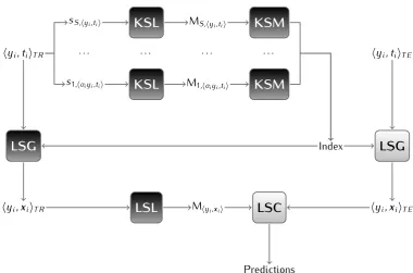
At a very high level, the feature projection process that we propose consists of three main tasks:

• We exploit the target kernel function in the original, high dimensional

space in combination with the SVM optimizer to carry out a first step of example selection and select the most relevant example points, i.e.

the support vectors. This step is called Kernel Space Learning (KSL),

since learning occurs in the space of the target kernel function;

• We use a greedy algorithm to explore the fragment space encoded by

the support vectors, generate the most relevant fragments and store

them into an index. We employ a gradient-based approach to decide

wich features to retain or discard, and also as a criterion to guide the greedy exploration of the fragment space. Indeed, fragments are selected based on their contribution to the norm of the gradient of the

model learnt during KSL. This stage is called Kernel Space Mining

(KSM);

• The index is used to decode the input structured data, i.e. the trees

in the dataset of the TK learning problem, and to represent them as

vectors in a linear space. This step is called Linear Space Generation

(58)

These three main building blocks can be combined in different ways, resulting in different architectures for tackling different learning problems or stress different properties of the feature selection methodology, as explained

in Section 4.1.

Gradient-based approaches to feature selection (see Section 3.2) exploit

the idea that a good variable selection strategy should have a limited effect on the geometry of the separating hyperplane, i.e. on the gradient. The contri