Performance Analysis of LMS Adaptive Beamforming Algorithm

(1)

International Journal of Electronics Communication and Computer Engineering Volume 4, Issue 5, ISSN (Online): 2249–071X,ISSN (Print): 2278–4209

Performance Analysis of LMS Adaptive Beamforming

Algorithm

Rupal Sahu, Mr. Ravi Mohan, Mr. Sumit Sharma

Abstract – The adoption of smart antenna techniques in future wireless systems is expected to have a significant impact on the efficient use of the spectrum, the minimization of the cost of establishing new wireless networks, the optimization of service quality, and realization of transparent operation across multi technology wireless networks.

This paper presents brief account on smart antenna (SA) system in context of adaptive beamforming particularly LMS. Further, Implementation that resolves around the LMS adaptive algorithm, chosen for its computational simplicity and high stability into the MATLAB simulation of an adaptive array of a smart antenna base station system, is to investigate its performance in the presence of multipath components and multiple users. The capabilities of smart / adaptive antenna are easily employable to Cognitive Radio and OFDMA system.

Keywords – Smart/Adaptive Antenna, Beam Forming, LMS, SDMA, OFDMA.

I. I

NTRODUCTION

Since Radio Frequency (RF) spectrum is limited and its efficient use is only possible by employing smart/adaptive antenna array system to exploit mobile systems capabilities for data and voice communication. The name smart refers to the signal processing capability that forms vital part of the adaptive antenna system which controls the antenna pattern by updating a set of antenna weights. Smart antenna, supported by signal processing capability, directs narrow beam towards desired users but at the same time introduces null towards interferers, thus optimizing the service quality and capacity. Consider a smart antenna system with (Ne) elements equally spaced (d) and user’s

signal arrives from desired angle 0 as shown in Fig 1 [1]. Adaptive beamforming scheme i.e. LMS is used to control weights adaptively to optimize signal to noise ratio (SNR)

of the desired signal in look direction Φ0.

Fig.1. Smart antenna array system

The array factor for elements (Ne) equally spaced (d) linear array is given by



_ _ _  _



  



cos 2

. )

(

d jn

ne

A AF

where α is the inter element phase shift and is described

as:

and Φ0is the desired direction of the beam.

In reality, antennas are not smart; it is the digital signal processing, along with the antenna, which makes the system smart. When smart antenna is deployed in mobile communication using either time division multiple access (TDMA) or code division multiple access (CDMA) environment, exploiting time slot or assigning different codes to different users respectively, it radiates beam towards desired users only. Each beam becomes a channel, thus avoiding interference in a cell.

Because of these, each coded channel reduces co-channel interference, due to the processing gain of the system. The processing gain (PG) of the CDMA system is described as:

PG= 10log (B / R b) (3)

where B is the CDMA channel bandwidth and R b is the information rate in bits per second.

If a single antenna is used for CDMA system, then this system supports a maximum of 31 users. When an array of five elements is employed instead of single antenna, then capacity of CDMA system can be increased more than four times. It can be further enhanced if array of more elements are used [2] [3] [4] [5] [6] [7].

II. B

EAMFORMING

Beamforming is a general signal processing technique used to control the directionality of the reception or transmission of a signal on a transducer array. Beam forming creates the radiation pattern of the antenna array by adding the phases of the signals in the desired direction and by nulling the pattern in the unwanted direction. The phases and amplitudes are adjusted to optimize the received signal. A standard tool for analyzing the performance of a beam-former is the response for a given N-by-1 weight vector W (k) as function of, known as the beam response. This angular response is computed for all possible angles.

III. A

DAPTIVE

B

EAMFORMING

The adaptive algorithm used in the signal processing has a profound effect on the performance of a Smart Antenna system. Although the smart antenna system is sometimes called the Space Division Multiple Access, it is not the Copyright © 2013 IJECCE, All right reserved

1377

Performance Analysis of LMS Adaptive Beamforming

Algorithm

Rupal Sahu, Mr. Ravi Mohan, Mr. Sumit Sharma

I. I

NTRODUCTION



_ _ _  _



  



cos 2

. )

(

d jn

ne

A AF

as:

PG= 10log (B / R b) (3)

II. B

EAMFORMING

III. A

DAPTIVE

B

EAMFORMING

The adaptive algorithm used in the signal processing has a profound effect on the performance of a Smart Antenna system. Although the smart antenna system is sometimes called the Space Division Multiple Access, it is not the Copyright © 2013 IJECCE, All right reserved

1377

Performance Analysis of LMS Adaptive Beamforming

Algorithm

Rupal Sahu, Mr. Ravi Mohan, Mr. Sumit Sharma

I. I

NTRODUCTION



_ _ _  _



  



cos 2

. )

(

d jn

ne

A AF

as:

PG= 10log (B / R b) (3)

II. B

EAMFORMING

III. A

DAPTIVE

B

EAMFORMING

(2)

antenna that is smart. The function of an antenna is to convert electrical signals into electromagnetic waves or vice versa but nothing else. The adaptive algorithm is the one that gives a smart antenna system its intelligence. Without an adaptive algorithm, the original signals can no longer be extracted. In the fixed weight beamforming approach the arrival angles does not change with time, so the optimum weight would not need to be adjusted. However, if desired arrival angles change with time, it is necessary to devise an optimization scheme that operates on-the-fly so as to keep recalculating the optimum array

weight that’s done by using adaptive beamforming

algorithm.

Fig.2. Block diagram of adaptive beamforming algorithm The task of the algorithm in a Smart antenna system is to adjust the received signals so that the desired signals are extracted once the signals are combined. Various methods can be used in the implementation of an adaptive algorithm.

In comparison, an human can even listen to sound which is weaker than the interference. The adaptive algorithm in a smart antenna system serves a similar purpose as the brain in this analogy, however it is less sophisticated. Our brain can perform the above signal selection and suppression with only two ears, but multiple antennas are required for the adaptive algorithm so that enough information on the user signals can be acquired to perform the task. In human beings, some people are more intelligent than others. In order for them to be more intelligent, they have to have a more developed brain. Similarly, some algorithms are smarter than other algorithms. A smart algorithm usually requires more resources than algorithms that are less intelligent. Unlike our brain which is a free resource, more resources in the world of technology always mean more expensive components and more complicated system.

IV. L

EAST

M

EAN

S

QUARE

A

LGORITHM

The Least Mean Square (LMS) algorithm, introduced by Widrow and Hoff in 1959 [3] [9] [10] is an adaptive algorithm, which uses a gradient-based method of steepest decent [8].

LMS algorithm uses the estimates of the gradient vector from the available data. LMS incorporates an iterative procedure that makes successive corrections to the weight vector in the direction of the negative of the gradient vector which eventually leads to the minimum mean square error.

Fig.3. LM S adaptive beamforming network A Uniform Linear Array (ULA) with N isotropic elements, which forms the integral part of the adaptive beamforming system, is shown [Fig-2].The output of the antenna array is given by,

) ( ) ( ) ( ) ( ) ( ) ( 1 t n a t u a t s t x u N i i i   



  

s(t) denotes the desired signal arriving at angleθₒand u(t) denotes interfering signals arriving at angle of incidences θi respectively. a(θ ) and a(θi) represents the steering vectors for the desired signal and interfering signals respectively. Therefore it is required to construct the desired signal from the received signal amid the interfering signal and additional noise n(t). The outputs of the individual sensors are linearly combined after being scaled using corresponding weights such that the antenna array pattern is optimized to have maximum possible gain in the direction of the desired signal and nulls in the direction of the interferers. The weights here will be computed using LMS algorithm based on Minimum Squared Error (MSE) criterion. Therefore the spatial filtering problem involves estimation of signal s(t) from the received signal x(t)(i.e. the array output) by minimizing the error between the reference signal d(t), which closely matches or has some extent of correlation with the desired signal estimate and the beamformer output y(t) (equal to wx(t)). This is a classical Weiner filtering problem for which the solution can be iteratively found using the LMS algorithm.

V. LMS A

LGORITHM

F

ORMULATION

From the method of steepest descent, the weight vector equation is given by

 







( )



2 1 ) ( ) 1

(n wn e2 n

w    

Where μ is the step-size parameter and controls the convergence characteristics of the LMS algorithm; e2(n) is the mean square error between the beamformer output y(n) and the reference signal which is given by,

e2(n) = [d (n)–w

h

x(n)]2

algorithm.

IV. L

EAST

M

EAN

S

QUARE

A

LGORITHM



  

s(t) denotes the desired signal arriving at angleθ and u(t) denotes interfering signals arriving at angle of incidences θi respectively. a(θ ) and a(θi) represents the steering vectors for the desired signal and interfering signals respectively. Therefore it is required to construct the desired signal from the received signal amid the interfering signal and additional noise n(t). The outputs of the individual sensors are linearly combined after being scaled using corresponding weights such that the antenna array pattern is optimized to have maximum possible gain in the direction of the desired signal and nulls in the direction of the interferers. The weights here will be computed using LMS algorithm based on Minimum Squared Error (MSE) criterion. Therefore the spatial filtering problem involves estimation of signal s(t) from the received signal x(t)(i.e. the array output) by minimizing the error between the reference signal d(t), which closely matches or has some extent of correlation with the desired signal estimate and the beamformer output y(t) (equal to wx(t)). This is a classical Weiner filtering problem for which the solution can be iteratively found using the LMS algorithm.

V. LMS A

LGORITHM

F

ORMULATION

 







( )



2 1 ) ( ) 1

(n wn e2 n

w    

e2(n) = [d (n)–w

h

x(n)]2

algorithm.

IV. L

EAST

M

EAN

S

QUARE

A

LGORITHM



  

s(t) denotes the desired signal arriving at angleθ and u(t) denotes interfering signals arriving at angle of incidences θi respectively. a(θ ) and a(θi) represents the steering vectors for the desired signal and interfering signals respectively. Therefore it is required to construct the desired signal from the received signal amid the interfering signal and additional noise n(t). The outputs of the individual sensors are linearly combined after being scaled using corresponding weights such that the antenna array pattern is optimized to have maximum possible gain in the direction of the desired signal and nulls in the direction of the interferers. The weights here will be computed using LMS algorithm based on Minimum Squared Error (MSE) criterion. Therefore the spatial filtering problem involves estimation of signal s(t) from the received signal x(t)(i.e. the array output) by minimizing the error between the reference signal d(t), which closely matches or has some extent of correlation with the desired signal estimate and the beamformer output y(t) (equal to wx(t)). This is a classical Weiner filtering problem for which the solution can be iteratively found using the LMS algorithm.

V. LMS A

LGORITHM

F

ORMULATION

 







( )



2 1 ) ( ) 1

(n wn e2 n

w    

e2(n) = [d (n)–w

h

(3)

The gradient vector in the above weight update equation can be computed as

In the method of steepest descent the biggest problem is the computation involved in finding the values r and R matrices in real time. The LMS algorithm on the other hand simplifies this by using the instantaneous values of covariance matrices r and R instead of their actual values i.e.

R(n) = x(n)x

h

(n) r(n) = d (n)x(n)

Therefore the weight update can be given by the following equation,

w(n+1) = w(n) + μx(n)[d (n)–x

h

(n)w(n) ] = w(n) + μx(n)e (n)

The LMS algorithm is initiated with an arbitrary value w (0) for the weight vector at n=0. The successive corrections of the weight vector eventually leads to the minimum value of the mean squared error.Therefore the LMS algorithm can be summarized in following equations;

Output, y(n)= w

h

x(n)

Error, e(n) = d⃰(n)–y(n) Weight, w(n+1) = w(n) + μx(n)e (n)

The LMS algorithm initiated with some arbitrary value for the weight vector is seen to converge and stay stable for

0 < μ < 1/λ

max

Whereλ

maxis the largest eigen value of the correlation matrix R. The convergence of the algorithm is inversely proportional to the eigenvalue spread of the correlation matrix R. When the eigenvalues of R are widespread, convergence may be slow. The eigenvalue spread of the correlation matrix is estimated by computing the ratio of the largest eigenvalue to the smallest eigenvalue of the matrix. Ifμ is chosen to be very small then the algorithm converges very slowly. A large value of μ may lead to a faster convergence but may be less stable around the minimum value.

VI. S

IMULATION

R

ESULTS FOR THE

LMS

A

LGORITHM

Table 1: Parameters used

Source Signal Angle 45º

Interference Signal Angle 60º

Signal to Noise Ratio (SNR) 15dB

Signal to Interference Ratio (SIR) 3 dB

LMS Step-size Parameter 0.05

Optimized-LMS Step-size Parameter 0.05

RLS Forgetting Factor 0.999

A linear 8 element array is simulated in MATLAB to analyse the results of LMS.

A simulation run of 100 iterations with parameters summarized in TABLE 1 resulted in error plot as shown in Fig.3. LMS algorithm exhibited a Brownian motion

around minimum value. To analyse the ability of algorithm to give maximum gain in the direction of source signal and placing the null in the direction of interference signal, simulations were performed using different interferer signal directions for 500 iterations. Remaining all parameters was set as mentioned earlier. Fig. 4, 5 and 6 shows polar and rectangular plots of LMS algorithms for interference signal arrival angle of 40º, 60º and 90º respectively.

For comparing the dependency of algorithm on SNR and SIR, it was compared at two values

• SNR=30dB, SIR=10dB

Fig.7 shows the behaviour of LMS algorithm respectively, for mentioned SNR and SIR values.

Fig.4. Error plot

Fig.5. Polar and Rectangular plot with interference signal at 40º

R(n) = x(n)x

h

(n) r(n) = d (n)x(n)

w(n+1) = w(n) + μx(n)[d (n)–x

h

(n)w(n) ] = w(n) + μx(n)e (n)

Output, y(n)= w

h

x(n)

Error, e(n) = d (n)–y(n) Weight, w(n+1) = w(n) + μx(n)e (n)

0 < μ < 1/λ

max

Whereλ

VI. S

IMULATION

R

ESULTS FOR THE

LMS

A

LGORITHM

Fig.4. Error plot

R(n) = x(n)x

h

(n) r(n) = d (n)x(n)

w(n+1) = w(n) + μx(n)[d (n)–x

h

(n)w(n) ] = w(n) + μx(n)e (n)

Output, y(n)= w

h

x(n)

Error, e(n) = d (n)–y(n) Weight, w(n+1) = w(n) + μx(n)e (n)

0 < μ < 1/λ

max

Whereλ

VI. S

IMULATION

R

ESULTS FOR THE

LMS

A

LGORITHM

Fig.4. Error plot

(4)

Fig.8. Polar and Rectangular of LMS algorithm

VII. C

ONCLUSION

The LMS algorithm is most commonly used

adaptive

algorithm because of its simplicity and a

reasonable performance. Since it is an iterative algorithm it can be used in a highly time-varying signal environment. It has a stable and robust performance against different signal conditions. However it may not have a really fast convergence speed compared other complicated algorithms like the Recursive Least Square (RLS). It converges with slow speeds when the environment yields a correlation matrix R possessing a large Eigen spread. Usually traffic conditions are not static, the user and interferer locations and the signal environment are varying with time, in which case the weights will not have enough time to converge when adapted at an identical rate. That is,

μ the step-size needs to be varied in accordance with the varying traffic conditions. It was found that the performance of the LMS beamformer improves as more elements are used in the antenna array. This improvement is seen in the form of sharper beams directed towards the desired users. Using small or large spacing values could degrade the performance of the LMS beamformer. It was also found that the performance improves as the angular separation between the incident signals increases. Moreover, it was noticed that increasing the number of elements of the antenna array ensures better performance towards signals with grazing incidence.

VIII. R

ESULT

In figure 9, we display the simulation result of smart antenna using direction of arrival (DOA) estimation and different adaptive beamforming ( MUSIC,MVDR and ESPRIT algorithm).

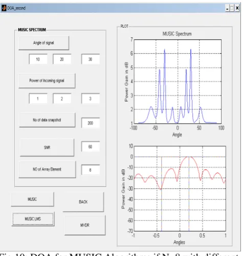
Fig.9. Display of DOA estimation for different algorithm In figure 10,we display the simulation result of smart antenna using direction of arrival (DOA) estimation and MUSIC algorithm for different angle and different power with SNR=60 and N=8 elements.

Fig 10: DOA for MUSIC Algorithms if N=8,with different angle & power

(5)

Fig.11. DOA for MVDR Algorithms if N=8, with different angle

Fig.12. DOA for ESPRIT Algorithms if N=8, with same angle

In figure 12, we display the simulation result of smart antenna using direction of arrival (DOA) estimation and ESPRIT algorithm for same angle with SNR=60 and N=8 elements.

R

EFERENCES

[1] LAL. C. GODARA, Senior Member, IEEE, “Applications of

Antenna Arrays to Mobile Communications, Part I; Performance Improvement, Feasibility, and System.

[2] LAL. C. GODARA, Senior Member, IEEE, “Applications of

Antenna Arrays to Mobile Communications, Part II;

Beam-Forming and Directional of Arrival Considerations,” Proceeding

of the IEEE, VOL. 85, NO. 8, pp. 1195-1245, August 1997. [3] Simon Haykin, Adaptive Filter Theory, third edition (New

Jersey, Prentice-Hall Inc., 1996).

[4] B. Widrow and S.D. Steams, Adaptive Signal Processing (New Jersey, Prentice-Hall Inc., 1985).

[5] Md. Bakhar, Dr. Vani R.M and Dr. P. V. Hunagund, “Eigen

Structure Based Direction of Arrival Estimation Algorithms for

Smart Antenna Systems,” IJCSNS International Journal of

Computer Science and Network Security, VOL. 9, NO. 11, pp. 96-100, November 2009.

[6] F. E. Fakoukakis, S. G. Diamantis, A. P. Orfanides and G. A.

kyriacou, “Development of an Adaptive and a Switched Beam Smart Antenna System for Wireless Communications,” Progress

in Electromagnetics Research Symposium 2005, Hangzhou, C hina, pp. 1-5, August 22-26, 2005.

[7] Rameshwar Kawitkar, “Issues in Deploying Smart Antennas in Mobile Radio Networks,” Proceedings of World Academy of

Science, Engineering and Technology Volume 31, July 2008, pp. 361-366, ISSN 1307-6884.

[8] Salvatore Bellofiore, Consfan fine A. Balanis, Jeffrey Foufz, and

Andreas S. Spanias, ―Smart-Antenna Systems for Mobile Communication Networks Part I: Overview and Antenna Design, IEEE Antenna’s and Propagation Magazine, Vol. 44,No. 3, June 2002.

[9] Bernard widrow, Semuel D. Stearns, ―Adaptive signal processing, Pearson education Asia, Second Indian reprint, 2002.

[10] Frank Gross, Smart Antenna for Wireless Communication, Mcgraw-hill, September 14, 2005.

[11] R. Martínez, A. Cacho, L. Haro, and M. Calvo “Comparative

study of LMS and RLS adaptive algorithms in the optimum combining of uplink W-CDMA”,IEEE, pp. 2258-2262, 2002.

[12] M. T. Islam, Z. A. Abdul Rashid, and C. C. Ping, “Comparison

between non-blind and blind array algorithms for smart antenna

system”,CS-2006-1015, pp. 1-8, 2006.

[13] R. S. Kawitkar and D. G. Wakde, “Smart antenna array analysis using LMS algorithm”,IEEE Int. Symposium on Microwave,

Antenna, Propagation and EMC Technologies for Wireless Communications, pp. 370-374, 2005.

[14] J. Razavilar, F. Rashid-Farrokhi, and K. J. R. Liu, “Software

radio architecture with smart antennas: a tutorial on algorithms

and complexity”, IEEE Journal on Selected Areas in Communications, Vol.17, No. 4, pp. 662-676, April 1999.

A

UTHOR

’

S

P

ROFILE

Rupal Sahu

is a PG scholar M. Tech. in microwave branch from RGPV Bhopal. Email: [email protected]

Mr. Ravimohan

is HOD in SRIT Jabalpur (MP) Email: [email protected]