A Survey on Shadow Detection Techniques in a Single Image

(1)

75

Information Technology and Control 2018/1/47

A Survey on Shadow Detection

Techniques in a Single Image

ITC 1/47

Journal of Information Technology and Control

Vol. 47 / No. 1 / 2018 pp. 75-92

DOI 10.5755/j01.itc.47.1.15012 © Kaunas University of Technology

A Survey on Shadow Detection Techniques in a Single Image

Received 2017/05/18 Accepted after revision 2018/01/12

http://dx.doi.org/10.5755/j01.itc.47.1.15012

Saritha Murali, Govindan V. K., Saidalavi Kalady

Department of Computer Science and Engineering, National Institute of Technology Calicut, Kerala, India. e-mails: [email protected], [email protected], [email protected]

Corresponding author: [email protected]

Shadows are inescapable elements in a scene formed due to the presence of an object between the light source and the surface on which it is cast. Appearance of shadows often causes severe issues in computer vision ap-plications like object extraction, and surveillance. Researchers have made effort to device techniques to locate and remove shadows from images and videos. This paper attempts to survey the various shadow detection al-gorithms for a single image. For the purpose of survey, the notable research work in the literature is classified under five major categories: invariant-based detection, feature-based detection, region-based detection, color model based detection and interactive shadow detection. The survey also includes a qualitative and quantita-tive evaluation of the methods discussed. As outcomes of the survey, it is observed that, (i) although the works discussed under each of these categories are capable of detecting shadows in different scenarios, the accura-cy and time taken need further improvements to make the shadow detection process acceptable for practical applications; (ii) detection of self-shadows and heavily scattered shadows is challenging; (iii) the risk of mis-classifying dark objects as shadows should be addressed; (iv) soft shadows that span multiple surfaces pose challenge in accurate detection of shadows.

KEYWORDS: Shadow detection, Invariant image, Feature extraction, Color models, Interactive.

1. Introduction

Shadows appear on a surface when light from a source (or multiple sources) is unable to reach the surface due to obstruction by an object. An object may cast shadow on itself (it is then called self-shadow), or on another surface (it is then termed as cast shadow). Al-though shadows can provide useful cues for estimat-ing scene illumination, findestimat-ing the geometry of object casting the shadow, locating the light source and so on,

(2)

The removal of shadows from an image can be con-sidered as a two-stage process, where the detection of shadows is to be performed first, followed by the removal. Most of the works in this area focus on shad-ows in video [4] and multiple images. Detection and elimination of shadows from a picture is troublesome since the entire cues for detection are to be derived from the single input image. An extensive review of cast shadow detection techniques depending on object/environment and domain was presented by Al-Najdawi et al. [1]. Different moving cast shadow ex-traction algorithms were studied by Sanin et al. [27]. They classified the algorithms under a feature-based taxonomy and performed a comparative analysis of the techniques. A major attempt in reviewing the shadow detection and removal from real images was done by Sasi and Govindan [29].

we present a brief shadow formation model in Section 2. Certain indicative properties of shadows are men-tioned in Section 3. This is succeeded by a critical re-view of different shadow detection algorithms, which are classified into five categories in Section 4. A qual-itative and quantqual-itative analysis is done in Section 5. We conclude the survey in Section 6.

2. The Shadow Formation Model

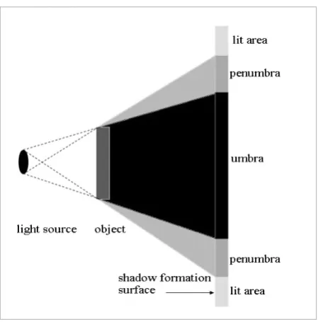
Figure 1 illustrates the formation of shadow due to the presence of an object between a non-point light source and the region where the shadow is cast upon. In this scenario, the shadow is seen to be comprised of two regions, the inner umbra and the outer penumbra. Umbra is the dark area in shadow formed by the complete obstruction of light, whereas, penumbra is the lighter area in the shadow formed due to partial blocking of direct light from the source. Since the illumination in the umbra region is much less com-pared to that in the penumbra and the lit area, it is the darkest shadow region. The texture detail in this region of shadow is mostly corrupted. The penumbra region looks much more diffused, but retains the tex-ture information. The main difficulty in locating the penumbra region arises due to the diffused boundary between the penumbra and the lit area.

An image may be considered to be a composition of two components that represent illumination and re-flectance [3]. The illumination component depends upon the light source which illuminates the scene, whereas, the reflectance element is based on the property of the surface or object which is illuminated. Hence, an image I(x,y) could be expressed as

�(�, �) � �(�, �) � �(�, �), (1)

Table 1

The properties of shadow regions and non-shadow regions

Property

Image 1 Image 2 Image 3

Value in Shadow area compared to Non-shadow S* NS* S NS S NS

RGB Values [95, 109, 121] [159, 168, 171] [64, 64, 58] [143, 132, 104] [73, 53, 52] [160, 113, 101] Lower Gray Level

Intensity 106 166 64 132 60 126 Lower

Local Max 152 249 101 226 82 201 Lower

Hue 0.58 0.50 0.16 0.13 0.22 0.03 Nearly same

Saturation 0.21 0.08 0.15 0.31 0.30 0.37 Lower

(1)

where R and L are the reflectance and the illumina-tion components, respectively. Since shadows are formed due to a lack of illumination, the removal of illumination component will provide a reflectance image which is nearly shadow-free.

3. The Properties of Shadows

Understanding the properties of shadows is inevita-ble in identifying the shadows in an image. Shadow Figure 1

Shadow formation model

(3)

77

regions exhibit various properties that differentiate them from the non-shadow areas in an image. The mean values of various properties for 64×64 patches

of shadow and corresponding non-shadow ground truth of three images from the dataset given in [16] are shown in Table 1.

Property Table 1

Property

Intensity 106 166 64 132 60 126 Lower

Local Max 152 249 101 226 82 201 Lower

Hue 0.58 0.50 0.16 0.13 0.22 0.03 Nearly same

Saturation 0.21 0.08 0.15 0.31 0.30 0.37 Lower Image 1

Table 1

Property

Intensity 106 166 64 132 60 126 Lower

Local Max 152 249 101 226 82 201 Lower

Hue 0.58 0.50 0.16 0.13 0.22 0.03 Nearly same

Table 1

Property

Intensity 106 166 64 132 60 126 Lower

Local Max 152 249 101 226 82 201 Lower

Hue 0.58 0.50 0.16 0.13 0.22 0.03 Nearly same

Value in Shadow area compared to Non-shadow

S* NS* S NS S NS

RGB Values [95, 109, 121] [159, 168, 171] [64, 64, 58] [143, 132, 104] [73, 53, 52] [160, 113, 101] Lower

Gray Level Intensity 106 166 64 132 60 126 Lower

Local Max 152 249 101 226 82 201 Lower

Hue 0.58 0.50 0.16 0.13 0.22 0.03 Nearly same

Saturation 0.21 0.08 0.15 0.31 0.30 0.37 Lower

Brightness 0.48 0.67 0.26 0.57 0.29 0.63 Lower

Entropy 5.44 6.51 5.76 7.10 4.23 5.32 Lower

Kurtosis 3.12 3.29 1.52 1.47 2.24 3.01 Different

Standard Deviation 10.61 22.47 20.47 54.73 6.21 16.16 Lower

Skewness 0.07 -0.02 0.32 0.24 0.37 0.88 Different

Graylevel Variance 112 504 419 2995 38 261 Lower

Table 1

*S- shadow NS- Non-shadow

It is observed that shadow regions have lower val-ues for RGB, graylevel intensity, standard deviation, variance, local maximum, and brightness since these values depend on the illumination and the shadow regions are less illuminated than the surroundings. The hue value that indicates the dominant color of a surface remains nearly the same in both shadow and shadowless regions [18]. Difference in skewness values arises due to difference in the asymmetries in shadow and non-shadow regions [41]. Since shadow areas are darker, their entropy [41] and saturation val-ues are less. Many of these properties are explored by the researchers to separate the shadow regions from the shadowless regions in an image.

4. Shadow Detection Methods

The initial stage in the elimination of shadows from an image involves correctly locating the shadow

ar-eas. Numerous works are available in the literature for detection of shadows in videos, aerial images, and outdoor images. In this paper, various techniques used for detecting the shadows in an image are dis-cussed.

We have identified five classes of detection algo-rithms:

A. Invariant-based shadow detection; B. Feature-based shadow detection

i. feature extraction based ii. feature learning based; C. Region-based shadow detection; D. Color model based shadow detection; E. Interactive shadow detection.

(4)

A. Invariant-Based Shadow Detection

Most of the early works in shadow detection from a single image focused on finding an invariant image rep-resentation in which shadows are absent or less visible. The theory of invariant image is based on the concept that shadows occur in lesser illuminated areas in an image. Hence, generating an illumination-invariant image could provide useful information on the shadow areas. Since shadows are absent in the invariant image, edge-map of illumination invariant image will have only object edges. The fundamental issue is to find a mechanism to generate such a representation.

The most prominent work in this category was done by Finlayson et al. [9]. They deployed a 1-Dimen-sional grayscale illumination-invariant represen-tation [8] of an image that is obtained by projecting the 2-Dimensional chromaticity along a line upright the direction of illumination change. Edge detec-tion was done on both illuminadetec-tion-invariant and original images. The differences in edge-maps of the images resulted in shadow edges. The problem with this method was in determining the direction of illu-mination change which required calibrated camer-as. Later, Finlayson et al. [7] demonstrated that the correct invariant direction is the one which will re-sult in least entropy in the 1-Dimensional greyscale invariant image. The 1-Dimensional invariant repre-sentation did not carry color information. Hence, a method to generate a 2- Dimensional invariant im-age that retains certain color information was put forward in [10]. He and Chu [17] used Fisher Linear Discriminant (FLD) to find the invariant direction. Even though the detection results are not that ac-ceptable, the authors verified that FLD can be used to generate invariant image. Two adjacent pixels on a surface form an illuminant discontinuity pair if they appear with dissimilar intensities in original image, but are aligned on same direction in the log chromaticity space. Lu and Drew [21] formulated an illuminant discontinuity measure,

kij= �<�_�� >

��‖��‖�� where �� is a vector that associates the log ratios of adjacent pixels i, j; and ��is the illuminant direction. This measure is obtained from intensity and chromaticity cues, and is used to label shadow pixels by Markov Random Field (MRF) with graph-cut optimization. Tian et al. [34] formulated a Tricolor Attenuation Model (TAM) considering the Spectral Power Distribution (SPD) of light during daytime and light from the sky to detect shadows in outdoor images. They developed an approximate shadow invariant by means of an RGB to greyscale transformation;

� = �� _{��[�}�� [�� ]

� �� ] + 1��

where [�� ] indicates the tricolor value of a pixel in an RGB image, and Y is the resultant grayscale image. This method works effectively on complex outdoor scenes also.

Discussion

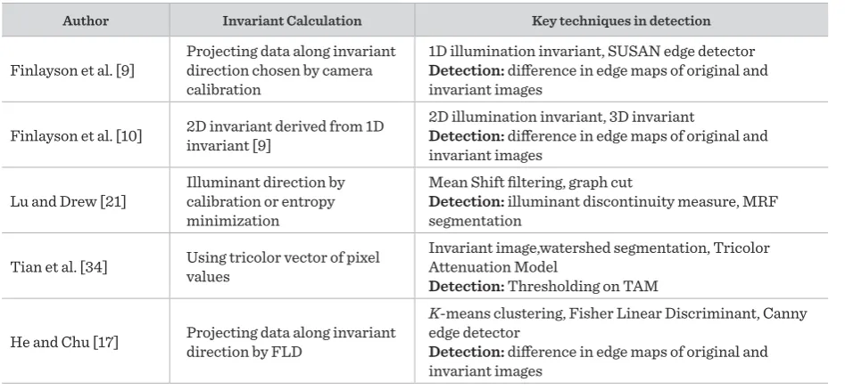
Invariant-based shadow detection techniques aim to find a representation that is free from shadows. These algorithms require prior knowledge of illuminant direction or calculation of illuminant direction by camera calibration [9], entropy minimization [7], or Fisher Linear discriminant [17]. Most of these algorithms work under the assumption of Planckian light, Lambertian surfaces and linear illumination. The generation of invariant images demands high quality input images that are noiseless and uncompressed. Detection results are also affected by the edge detection algorithms used to create the edgemap of the original image and its invariant. However, these methods generally incur less time for generating the results. A summary of the features of the algorithms mentioned in this category is included in Table 2.

Table 2

A summary of invariant based shadow detection methods

Author Invariant Calculation Key techniques in detection

Finlayson et al. [9] Projecting data along invariant direction chosen by camera calibration

1D illumination invariant, SUSAN edge detector Detection: difference in edge maps of original and invariant images

Finlayson et al. [10] 2D invariant derived from 1D

invariant [9] 2D illumination invariant, 3D invariant Detection: difference in edge maps of original and invariant images

Lu and Drew [21] Illuminant direction by calibration or entropy minimization

Mean Shift filtering, graph cut

Detection: illuminant discontinuity measure, MRF segmentation

Tian et al. [34] Using tricolor vector of pixel

values Invariant image,watershed segmentation, Tricolor Attenuation Model Detection: Thresholding on TAM

He and Chu [17] Projecting data along invariant

direction by FLD Kedge detector -means clustering, Fisher Linear Discriminant, Canny Detection: difference in edge maps of original and invariant images

(2)

where e_ij is a vector that associates the log ratios of adjacent pixels i, j; and e0 is the illuminant direction.

This measure is obtained from intensity and chro-maticity cues, and is used to label shadow pixels by Markov Random Field (MRF) with graph-cut optimi-zation. Tian et al. [34] formulated a Tricolor Attenu-ation Model (TAM) considering the Spectral Power Distribution (SPD) of light during daytime and light from the sky to detect shadows in outdoor images. They developed an approximate shadow invariant by means of an RGB to greyscale transformation;

kij= �<�_�� >

��‖��‖��

where �� is a vector that associates the log ratios of adjacent pixels i, j; and ��is the illuminant direction.

This measure is obtained from intensity and chromaticity cues, and is used to label shadow pixels by Markov Random Field (MRF) with graph-cut optimization. Tian et al. [34] formulated a Tricolor Attenuation Model (TAM) considering the Spectral Power Distribution (SPD) of light during daytime and light from the sky to detect shadows in outdoor images. They developed an approximate shadow invariant by means of an RGB to greyscale transformation;

� = �� _{��[�}�� [�� ]

� �� ] + 1��

where [�� ] indicates the tricolor value of a pixel in an RGB image, and Y is the resultant grayscale

image. This method works effectively on complex outdoor scenes also.

Discussion

Invariant-based shadow detection techniques aim to find a representation that is free from shadows. These algorithms require prior knowledge of illuminant direction or calculation of illuminant direction by camera calibration [9], entropy minimization [7], or Fisher Linear discriminant [17]. Most of these algorithms work under the assumption of Planckian light, Lambertian surfaces and linear illumination. The generation of invariant images demands high quality input images that are noiseless and uncompressed. Detection results are also affected by the edge detection algorithms used to create the edgemap of the original image and its invariant. However, these methods generally incur less time for generating the results. A summary of the features of the algorithms mentioned in this category is included in Table 2.

Table 2

1D illumination invariant, SUSAN edge detector Detection: difference in edge maps of original and invariant images

Finlayson et al. [10] 2D invariant derived from 1D

invariant [9] 2D illumination invariant, 3D invariant Detection: difference in edge maps of original and invariant images

Detection: illuminant discontinuity measure, MRF segmentation

Tian et al. [34] Using tricolor vector of pixel

values Invariant image,watershed segmentation, Tricolor Attenuation Model Detection: Thresholding on TAM

He and Chu [17] Projecting data along invariant

direction by FLD Kedge detector -means clustering, Fisher Linear Discriminant, Canny Detection: difference in edge maps of original and invariant images

(3)

where [FR FG FB] indicates the tricolor value of a pixel

in an RGB image, and Y is the resultant grayscale im-age. This method works effectively on complex outdoor scenes also.

Discussion

Invariant-based shadow detection techniques aim to find a representation that is free from shadows. These algorithms require prior knowledge of illumi-nant direction or calculation of illumiillumi-nant direction by camera calibration [9], entropy minimization [7], or Fisher Linear discriminant [17]. Most of these al-gorithms work under the assumption of Planckian light, Lambertian surfaces and linear illumination. The generation of invariant images demands high quality input images that are noiseless and uncom-pressed. Detection results are also affected by the edge detection algorithms used to create the edge-map of the original image and its invariant. Howev-er, these methods generally incur less time for gen-erating the results. A summary of the features of the algorithms mentioned in this category is included in Table 2.

B. Feature-Based Shadow Detection

(5)

79

two subsections, namely feature extraction based de-tection and feature learning based dede-tection.

i. Feature Extraction Based Shadow Detection

By using a single feature it is often difficult to iden-tify whether a pixel or region belongs to shadow or non-shadow region. Therefore, most of the feature extraction based algorithms intent to determine the best combination of features that can correctly detect the shadow regions in an image.

Salvador et al. [26] modelled shadow detection as a multi-stage process using color invariant and geomet-ric features. The algorithm begins by testing a hypoth-esis formulated over the concept that shadows black-en the area on which they are formed. This is followed by a verification of the result using color invariance and shadow location with reference to the object. The color invariant used in their technique was c1c2c3 model [11]. The method often fails to determine the shadow lines for soft shadows. A method to locate shadows using a combination of colour and edge fea-tures was put forward by Golchin et al. [13]. Shadow pixels were detected in HSI, modified c1c2c3, YCbCr color spaces, and hue difference of the background and the foreground regions separately. Followed by this, detection was done based on edge information Table 2

1D illumination invariant, SUSAN edge detector

Detection: difference in edge maps of original and invariant images

Finlayson et al. [10] 2D invariant derived from 1D _{invariant [9]} 2D illumination invariant, 3D invariantDetection: difference in edge maps of original and invariant images

Detection: illuminant discontinuity measure, MRF segmentation

Tian et al. [34] Using tricolor vector of pixel _values Invariant image,watershed segmentation, Tricolor Attenuation Model

Detection: Thresholding on TAM

He and Chu [17] Projecting data along invariant _{direction by FLD}

K-means clustering, Fisher Linear Discriminant, Canny edge detector

Detection: difference in edge maps of original and invariant images

using Sobel operator. Finally, all the detection results were combined using Boolean AND. Even though the method requires the background image as extra input, it is found to outperform the detection using color or edge feature alone.

Detection of shadows by using bright channel is an-other work in this category. The concept of a bright channel lies on the assumption that any image seg-ment will have pixels with values close to the in-coming radiance in at least one color channel. Pa-nagopoulos et al. [24] used this property to extract shadows from an image. The bright channel formed is refined by computing confidence of shadow areas using shadow features such as hue or by using Mar-kov Random Field (MRF) model. The refined bright channel is then threshold into a binary image to get the shadow regions.

(6)

over-exposed or noisy shadow regions. Dong et al. [5] attempted to model soft shadows using three fea-tures – center, orientation and width of penumbra. These measures were derived by fitting the intensity changes to a sigmoid function, and were used to de-tect shadows. The major pitfall of this method is the difficulty in detecting shadows on multiple surfaces and uneven surfaces.

ii. Feature Learning Based Shadow Detection

The feature based techniques that use a trained clas-sifier to separate the shadow and shadowless regions are discussed in this section. Some of these works use a predefined set of features for training while others automatically learn the most relevant features for classification.

Gijsenij and Gevers [12] experimentally proved that a unification of geometric and photometric features could enhance the detection results compared to us-ing either of the features alone. They used a nearest neighbour classifier to identify shadow patches in an image based on photometric and geometric features. The results show that the best geometric features that aid in detection are diagonal edges or absence of edges in the patch.

A method to detect shadows cast on ground was pro-posed by Lalonde et al. [20]. Initially, a decision tree classifier is trained on the basis of various color and

Author Features Key techniques in detection

Salvador et al. [26] Spectral (color invariance) and _{geometric features} Sobel operator, photometric color invariant features, spatial constraints.

Detection:Thresholding

Panagopoulos et al. [24] Bright channel cue,illumination invariant features: Hue, normalized RGB, c1c2c3

Bright channel, Markov Random Field

Golchin et al. [13] Color Features: HSI, modified

c1c2c3,YCbCr, hue difference Edge Features

Sobel operator, Morphological open operator

Dong et al. [5] Soft shadow features: center position, orientation and width of penumbra

Watershed segmentation, Canny edge detector, level-set optimization

Detection: intensity fitting

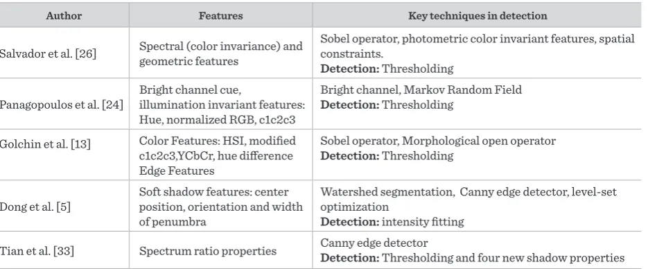
Tian et al. [33] Spectrum ratio properties Canny edge detector _Detection:_{Thresholding and four new shadow properties} Table 3

A summary of feature extraction based shadow detection methods

intensity features computed around the image edges. A 48-dimensional feature vector is generated for each pixel. Conditional Random Field (CRF) incorporated with a scene layout descriptor is then used to group the detected shadow edges. The method often fails for shadows of thin objects.

Zhu et al. [41] formulated a feature learning method to locate shadows in a monochromatic image. They used such shadow variant features as intensity difference, local max, smoothness and skewness; such shadow-in-variant features as gradient similarity and texture sim-ilarity; and such near black features as discrete entropy and edge response to train the classifier. Each pixel is labelled as shadow or not based on classifier built by integrating Boosted Decision Tree (BDT) with binary CRF (BCRF). The authors conclude that the integrated classifier outperforms BDT or BCRF alone.

(7)

region-81

al and across-boundary features using two different ConvNets (Convolutional deep Neural Networks). The unary and pairwise potentials of these features are combined in a CRF framework and shadow label-ling is done using Maximum a Posteriori (MAP) esti-mate. A method to learn the most important structure features of shadow boundaries using a structured Convolutional Neural Network (CNN) framework was given by Shen et al. [31]. The authors introduced shadow and bright values to approximately construct the complicated relation among the image regions. Shadow detection is formulated as a least square op-timization of non-local region constraints.

Discussion

The feature-based techniques for shadow detection provide best results when the optimal set of features is correctly identified. Determining this optimal set

Table 4

A summary of feature learning based shadow detection methods

Author Features Key techniques in detection

Gijsenij et al. [12]

Photometric: Quasi-invariants, Physics-based invariants, Color constancy at pixel, Normalized-RGB.

Geometric: SIFT,LBP,GLCM

Maximum posterior probability

Classifier: Nearest-neighbour

Lalonde et al. [20] Boundary features: brightness ratios, color intensity ratios, texture, skewness, edge sharpness, scene layout cues

Bilateral filter, watershed segmentation, Canny edge detector, CRF optimization

Classifier: logistic regression of Adaboost decision tree

Zhu et al. [41]

Shadow-variant: intensity difference, local max, smoothness, skewness

Shadow-invariant: gradient, texture similarity near black features: discrete entropy, edge response

MRF labeling

Classifier: Boosted decision tree with binary CRF

Wu et al. [37]

Illumination invariant: reflectance, color variance, gradient entropy

Illumination direction: 2D log chromaticity Neighbouring similarity: gradient, texton

Adaptive gradient threshold to get edge candidates, Spatial patch smoothing

Classifier: SVM

Khan et al. [19] Regional and across-boundary features

SLIC superpixel extraction ,gPb boundary detector, MAP estimate, CRF labeling

Classifier: 2 CNNs to detect shadow regions and edges

Shen et al. [31] Local structure information of shadow edge Canny edge detector, shadow/bright measure, Quick Shift segmentation

Classifier: structured CNN

(8)

C. Region-Based Shadow Detection

Traditional methods for shadow detection consid-ered it to be a pixel-labeling or edge-classification problem. Later, the region-based techniques evolved in which the segmented regions in an image were la-beled as shadows or non-shadows based on the prop-erties of individual regions as well as similarity with other regions. The single region classification consid-ers features like color, texture, and brightness, where-as pairwise clwhere-assification is done by comparing the properties of two regions such as histograms of color and texture, intensity ratios, chromatic alignment, and distance between them. The major works in re-gion-based detection are examined in this section. Guo et al. [16] modeled a region based technique to detect shadows from natural scenes. They trained a single region classifier using SVM with χ2 kernel and a pairwise classifier using SVM with RBF ker-nel. An energy function that integrates the single region classifier and pairwise classifier predictions was then minimized by using graph cut. Their pair-wise classifiers compare regions of same material with same illumination and different illumination. The key advantage of this method is that the pair-wise classifier considers non-adjacent regions also. Yuan et al. [40] used a physical model called color shade descriptor [30] in L*a*b* color space to find pairwise potentials of shadow regions. The descrip-tor is based on scene reflectance. Logistic regression of Adaboost with 16-node decision trees is trained for single region classification. These singleton and pairwise potentials are incorporated into a Condi-tional Random Field (CRF) model. The method per-forms poorly when the surface is uneven or is defi-cient in color information.

An SVM classifier with multi-kernel model was used to learn individual shadow regions in the work by Vi-cente et al. [35]. Their multi-kernel model is an inte-gration of the separate kernels for each feature. The pairwise classifiers used in this method compare only the adjacent regions of same material with same and different illumination. A boundary classifier was also introduced to deal with the shadow boundaries on a surface. All these classifiers are further optimized in an MRF framework. Similar to [16], this approach also gives same weight to all features computed. A region-based shadow detection technique that

learns the feature weights along with the classifier was proposed by Vicente et al. [36]. They trained a Least Square Support Vector Machine (LS-SVM) to find the probability of each region to be a shadow region, and contextual relation between neighboring regions to find the pairwise potential. The labeling was optimized by minimizing the leave-one-out error. The classical split-and-merge algorithm with fuzzy predicate was used to detect shadow regions in Sasi and Govindan [28]. The method splits and merges adjacent homogeneous quadtree blocks in the image based on the predicate. Entropy, edge response, stan-dard deviation, and mean of quadtree blocks were considered for building the fuzzy predicate.

Discussion

The key idea behind region-based shadow detection techniques is that the correctness of detection can be improved by incorporating a pairwise classifier that classifies a region into shadow or non-shadow by comparing it with the other regions in the image. Techniques that compare adjacent regions only and those that consider non-adjacent regions were men-tioned in this section. Most of these algorithms work on the basis of learned region features. Hence, the computational load is generally high for this category of algorithms. Table 5 consolidates the single region features and pairwise features considered for these methods and the classifiers used for detection. D. Color-Model Based Shadow Detection Transforming an image from one color model to an-other may provide vital cues for detecting shadows in it. The color model based shadow detection tech-niques initially convert an RGB image to another color model followed by detection in the new model. Normalized RGB, c1c2c3 and HSV are the most com-monly used color models for shadow detection since they produce image invariant to shadows. Other color spaces used are CIEL*u*v* and CIEL*a*b* due to their similarity with human perception.

(9)

af-83

fected by shadows. The dark regions in both the cas-es are then classified into self-shadow or cast shad-ow based on their presence in object contours. This method works for shadows cast on a flat, non-tex-tured surface only, and the object casting the shadow is expected to be within the image. Figov et al. [6] used a multi-resolution approach in which Fuzzy C-means clustering followed by shadow segmentation is done on a lower resolution CIEL*u*v* color representation of the image. This segmentation is then incorporat-ed to the original image to identify the shadow areas. They used a simple Euclidean distance measure to identify regions with similar chrominance and vary-ing luminance given in Equation (4):

�|(� �� )|� � �(� �)�_{+(� �)}�_{+(� �)}�_{. (4)}₍₄₎

Since a reduced size image is used, the algorithm demands that the original image should not be over-compressed.

An attempt to identify vague and hard shadows from an image was done by Xu et al. [39]. For identify-ing hard shadows, normalized RGB (L2 norm) and a 1-Dimensional invariant image generated by using [10] were used. The vague shadows were detected by thresholding the image gradient. The normalized RGB was computed as follows:

Author Classifier Features

Guo et al. [16] Single region:_Pairwise:_{SVM with RBF kernel} SVM with χ2 kernel; Single region: Pairwise: Color and texture histogram distances, intensity Color and texture histograms ratio, chromatic alignment, distance

Vicente et al. [35] Single-region: Boundary, pairwise classifiersmultikernel SVM;: SVM (RBFkernel)

Single region: Color and texture histograms

Pairwise: distances between color and texture histograms

Yuan et al. [40] Single-region: decision trees; logistic regression,

Pairwise: color shade descriptor

Single region: Color, brightness and texture histograms

Pairwise: Local maxima of color distribution

Vicente et al. [36] Single-region: _Pairwise:_{Contextual cues}Least Square SVM Single region: _Pairwise:_{Color and texture histogram distances, RGB ratios}Color, intensity, texture histograms

Sasi and

Govindan [28] Fuzzy Split and Merge using Adaptive Neuro-Fuzzy Inference System Entropy, edge response, standard deviation, mean of quadtree Table 5

A summary of region based shadow detection methods

��₌ �

��_��_��, (5)

��₌ �

��_��_��, (6)

��₌ �

��_��_��. (7) The detected shadow masks are combined to form reintegrated shadow mask.

Murali and Govindan [22] detected shadows in CIE L*a*b* color space based on luminance value and observed that the B-channel values (yellow to blue ratio) are lesser in shadow regions compared to the shadow regions. This method gives spurious labeling since it classifies each pixel as shadow and non-shadow without considering the neighboring pixels.

Discussion

The primary focus of color model based detection techniques is to identify cues that can aid in detecting shadows in a color space different from that of the original image. Color models L*a*b* and L*u*v* have separate luminance component that makes them useful for this purpose. While the algorithms that use color models are simple and fast, most of them misclassify dark regions in the image as shadows. The major features are summarised in Table 6.

E. Interactive Shadow Detection

Fully automatic shadow detection is yet a challenging problem primarily due to the difficulty in determining whether an area in an image is dark by itself or due to shadow cast on it. Interactive shadow detection techniques let the users incorporate their knowledge in the detection task. This section gives a brief review of five shadow detection techniques that need user input.

Wu and Tang [38] proposed a shadow extraction technique based on quadmap input by the user. The Table 6

A summary of color model based shadow detection methods

Author Color model Key techniques in detection

Figov et al. [6] CIE L*u*v* Segment features: area, border length, intensity with respect to neighbor segments, color ratio, brightness ratio

- Fuzzy c-means clustering Salvador et al. [25] c1c2c3 color invariant Luminance and color information Xu et al. [39] normalized RGB

(L2 norm)

Vague shadows: gradient thresholding; Hard shadows: color invariant thresholding - 1D invariant image, Gaussian smooth filter Murali and Govindan [22] CIE L*a*b* Thresholding on L and B channel values

(5)

��₌ �

��_��_��, (5)

��₌ �

��_��_��, (6)

��₌ �

��_��_��. (7)

The detected shadow masks are combined to form reintegrated shadow mask.

Discussion

E. Interactive Shadow Detection

(L2 norm) Vague shadows: gradient thresholding; Hard shadows: color invariant thresholding - 1D invariant image, Gaussian smooth filter Murali and Govindan [22] CIE L*a*b* Thresholding on L and B channel values

(6)

��₌ �

��_��_��, (5)

��₌ �

��_��_��, (6)

��₌ �

��_��_��. (7) The detected shadow masks are combined to form reintegrated shadow mask.

Discussion

E. Interactive Shadow Detection

(L2 norm) Vague shadows: gradient thresholding; Hard shadows: color invariant thresholding - 1D invariant image, Gaussian smooth filter Murali and Govindan [22] CIE L*a*b* Thresholding on L and B channel values

(7)

The detected shadow masks are combined to form re-integrated shadow mask.

Murali and Govindan [22] detected shadows in CIE L*a*b* color space based on luminance value and ob-served that the B-channel values (yellow to blue ratio) are lesser in shadow regions compared to the non-shad-ow regions. This method gives spurious labeling since it classifies each pixel as shadow and non-shadow without considering the neighboring pixels.

Discussion

(10)

col-or models are simple and fast, most of them misclas-sify dark regions in the image as shadows. The major features are summarised in Table 6.

E. Interactive Shadow Detection

Fully automatic shadow detection is yet a challenging problem primarily due to the difficulty in determining whether an area in an image is dark by itself or due to shadow cast on it. Interactive shadow detection tech-niques let the users incorporate their knowledge in the detection task. This section gives a brief review of five shadow detection techniques that need user input.

Wu and Tang [38] proposed a shadow extraction technique based on quadmap input by the user. The quadmap requires the user to mark four different re-gions in an image: shadow, non-shadow, uncertain and excluded regions. This input is used in a Bayesian framework to extract the shadow. A method to find shadows in outdoor image with a reduced user input was given by Nielsen and Madsen [23]. In this ap-Table 6

Figov et al. [6] CIE L*u*v* Segment features: area, border length, intensity with respect to neighbor segments, color ratio, brightness ratio - Fuzzy c-means clustering

Salvador et al. [25] c1c2c3 color invariant Luminance and color information

Xu et al. [39] normalized RGB _{(L2 norm)} Vague shadows: gradient thresholding; Hard shadows: color invariant thresholding - 1D invariant image, Gaussian smooth filter

Murali and Govindan [22] CIE L*a*b* Thresholding on L and B channel values

proach, the user should mark a shadow surface and its sunlit counterpart which is used to compute an alpha parameter. The shadow region is modeled as a func-tion of sunlit region using an alpha overlay and the edges were detected by thresholding based on inten-sity and illuminant direction. The method often fails for high frequency texture surface.

In the shadow detection technique by Arbel and Hel-Or [2], region growing using SVM is done separately on the multiple shadow and non-shadow coordinates input by the user. These detected shadow regions are later combined to form the shadow mask. The detec-tion becomes difficult for highly broken shadows, and those on multiple surfaces. One of the simplest inter-active methods was proposed by Shor and Lischinski [32] in which the user had to indicate the shadow re-gion by a bare mouse click. The shadow mask is de-rived from the clicked area by iterative region grow-ing and an illumination invariant distance measure. This technique works only for a surface which has

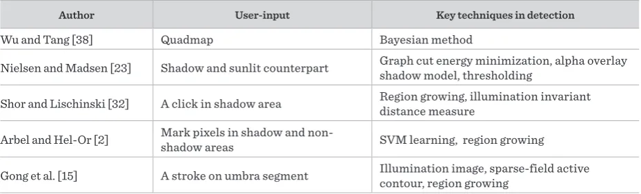
Table 7

Summary of interactive shadow detection methods

Author User-input Key techniques in detection

Wu and Tang [38] Quadmap Bayesian method

Nielsen and Madsen [23] Shadow and sunlit counterpart Graph cut energy minimization, alpha overlay _{shadow model, thresholding}

Shor and Lischinski [32] A click in shadow area Region growing, illumination invariant _{distance measure}

Arbel and Hel-Or [2] Mark pixels in shadow and non-_{shadow areas} SVM learning, region growing

(11)

85

both shadowed and non-shadowed areas.

A recent work by Gong et al. [15] requires the user to highlight a portion of umbra by one rough stroke. The segment was then used to detect shadow boundar-ies by region growing on an illumination image con-structed from HSV, LUV, and YCbCr color spaces. The method is found to work well for non-uniform umbra illumination.

Discussion

In general, the interactive shadow detection tech-niques are simpler than automatic detection since an initial indication of shadow region is provided by the user. However, these methods become annoying for the user if the image has multiple disjoint shad-ow regions. In this case, the user should give hint on each disjoint shadow region. Since the user himself/ herself provides clue on the shadow regions, there is less chance of misclassifying dark objects that are non-adjacent to shadow regions. The techniques dis-cussed are outlined in Table 7.

5. Comparison

This section begins with a concise explanation of the most widely used shadow detection datasets. This is succeeded by a comparison of the various shadow de-tection techniques discussed above. The comparison is done both qualitatively and quantitatively.

Shadow Detection Datasets

The major datasets available for shadow detection and removal in single images are listed below:

1 UCF dataset: 355 images and corresponding

man-ually-labeled ground truths given by [41].

2 UIUC dataset: 108 natural scenes taken under

dif-ferent illumination and their ground truth by [16].

3 CMU dataset: 135 outdoor images with shadow

boundary annotations given by [20].

4 Dataset by [14]: 214 images with ground truth.

Qualitative Analysis

Some of the works in literature consider shadow de-tection as a pixel-labeling problem, while others per-form detection at patch-level, region-level or edge lev-el. A qualitative summary of the algorithms discussed

under each category is given in Table 8. Furthermore, successful and failure cases in shadow detection un-der different scenarios are demonstrated in Table 9 and Table 10. Table 9(a) gives a comparison of the de-tection results of shadow region-growing technique and pixel-based detection. It is observed that the pix-el-labeling technique used by [22] gives spurious re-sult since the method considers properties of individ-ual pixels without considering the neighboring pixels during classification.

Many of the techniques impose constraints on the image quality, lighting conditions, and surface prop-erties. Some of the detection techniques need the in-put image to be segmented using standard algorithms. Watershed segmentation was used in [34, 5] and [20]. In these cases, the quality of shadow detection de-pends on the segmentation algorithm adopted. In ad-dition, edge detectors such as Canny [10, 17, 33, 5, 31], SUSAN [9, 20], and Sobel [26, 13] were used for initial edge detection in a few works. The inaccuracies in the edge detection also contribute to spurious edges in shadow detection results. Table 9(b)(iii) illustrates a case where Canny edge detector was used to extract edges. Another example for spurious edges is given in Table 9(c)(iii). Dependence on the surface properties is another criterion that aids in comparison of shad-ow detection algorithms. A situation where detection fails due to unusual surface color is shown in Ta-ble 9(d)(iii). This happened since Lalonde et al. [20] used a learning-based technique to locate shadows present in outdoor images where the training set was built with images in which materials constituting the surface are expected to be made of selected materials only. Surface geometry also contributes to efficient shadow detection [40].

An example of dark region misclassification is given in Table 9(e)(iii). The input image has an object which has a dark area similar to the color of shadows in the image. This has led to the misclassification by Guo et al. [16]. Conversely, the feature learning method proposed by Shen et al. [31] was able to classify the non-shadow regions correctly. Dark region misclassi-fication for large dark areas occurs in the method by Panagopoulos et al. [24].

(12)

Table 8

A qualitative summary of shadow detection methods

Invariant based level SD SS HS DS DM LD SR ER L

Finlayson et al. [9] pixel ✕ ✓ ✓ ✓ ✕ ✓ ✕

Finlayson et al. [10] pixel ✕ ✓ ✓ ✓ ✕ ✓ ✕

Lu and Drew [21] pixel ✕ ✓ ✓ ✓ ✕ ✕ ✕

Tian et al. [34] region ✓ ✓ ✓ ✕ ✓ ✕ ✕ ✕

He and Chu [17] pixel ✓ ✓ ✕ ✕ ✓ ✓ ✓ ✕

Feature Extraction based level SD SS HS DS DM LD SR ER L

Salvador et al. [26] pixel ✕ ✓ ✓ ✕ ✕ ✕ ✓ ✕

Panagopoulos et al. [24] patch ✓ ✓ M ✓ ✕ ✕ ✕

Golchin et al. [13] pixel ✓ ✓ ✓ ✕ ✕ ✓ ✕

Dong et al. [5] edge ✓ ✓ ✓ ✕ ✓ ✓ ✓ ✕

Tian et al. [33] edge ✕ ✕ ✓ ✓ ✕ ✓ ✕ ✓ ✕

Feature learning based level SD SS HS DS DM LD SR ER L

Gijsenij et al. [12] patch ✓ ✓ ✓ ✓

Lalonde et al. [20] edge ✕ ✓ ✓ ✓ ✓ ✓ ✓ ✓

Zhu et al. [41] pixel ✓ ✓ ✕ ✕ ✕ ✕ ✓

Wu et al. [37] patch ✕ M ✓ ✓ ✓ ✕ ✕ ✓

Khan et al. [19] pixel ✕ ✓ ✓ ✕ ✓ ✕ ✕ ✕ ✓

Shen et al. [31] patch ✓ ✓ ✓ ✕ ✓ ✓ ✓

Region based level SD SS HS DS DM LD SR NR L

Guo et al. [16] region ✓ ✓ ✓ ✕ ✓ ✓ ✓ ✓ ✓

Vicente et al. [35] region ✕ ✓ ✓ ✓ ✕ ✓

Yuan et al. [40] region ✕ ✓ ✓ ✓ ✓ ✓ ✓ ✕ ✓

Vicente et al. [36] region ✓ ✓ ✓ ✕ ✓ ✓ ✕ ✓

Sasi and Govindan [28] region ✓ ✓ ✓ ✕ ✕ ✕ ✕ ✓

Color model based level SD SS HS DS DM LD SR ER L

Salvador et al. [25] edge ✓ ✓ ✓ ✓ ✓ ✓ ✕

Figov et al. [6] segment ✕ ✕ ✓ ✓ ✓ ✓ ✕ ✕

Xu et al. [39] edge ✓ ✓ ✓ ✕ ✕ ✕

Murali and Govindan [22] pixel ✓ ✓ ✓ ✓ ✓ ✕ ✕ ✕

Interactive based level SD SS HS DS DM LD SR ER L

Wu and Tang [38] pixel ✓ ✓ ✓ ✕ ✕

Nielsen and Madsen [23] pixel ✓ ✓ ✓ ✕ ✓ ✕

Shor and Lischinski [32] pixel ✓ ✓ ✓ ✓ ✓ ✕

Arbel and Hel-Or [2] pixel ✓ ✓ ✓ ✓ ✓

Gong et al. [15] region ✓ ✓ ✓ ✕ ✕

(13)

87

Table 9

Shadow Detection – Qualitative results I: Row (i) has input images; (ii) and (iii) are detection results indicating success and failure cases respectively from the work mentioned under each image. Shadow regions/edges are represented as white in detection outputs (ii) and (iii)

(a) Region vs

Pixel-based on edge detection(b) Dependence (c) Spurious edges dependence(d) Surface misclassification(e) Dark region (f) Self-shadow detection

(i)

input image input image input image input image input image input image

(ii)

Gong et al. [15] Lu and Drew [21] Figov et al. [6] Shen et al. [31] Shen et al. [31] Guo et al. [16]

(iii)

Murali and

Gov-indan [22] He and Chu [17] Finlayson et al. [8] Lalonde et al. [20] Guo et al. [16] Yuan et al. [40]

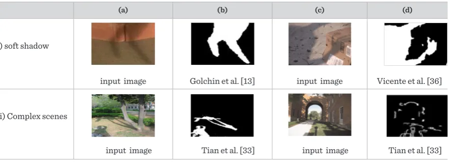
Table 10

Shadow Detection – Qualitative results II: Columns (a) and (c) are input images; (b) and (d) are detection results indicating success and failure cases respectively from the work mentioned under each image. Shadow region/edges are represented as white in (b) and (d)

(a) (b) (c) (d)

(i) soft shadow

input image Golchin et al. [13] input image Vicente et al. [36]

(ii) Complex scenes

input image Tian et al. [33] input image Tian et al. [33]

challenge in accurate detection of shadows [5]. Table 10(d)(i) illustrates the case in which extended soft shadows were undetected due to error in the ini-tial segmentation since soft shadow boundaries are

not detected by most of the segmentation or edge de-tection algorithms.

(14)

Information Technology and Control 2018/1/47 88

with very less misclassification. Table 10(d)(ii) is a failure case due to overexposed regions.

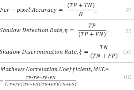
Quantitative Analysis

Numerous metrics are available for evaluating the correctness of shadow detection results. Most of the authors use Per-pixel accuracy, Shadow Detection Rate, and Shadow Discrimination Rate. Matthews Correlation Coefficient (MCC) was used by Sasi and Govindan [28]. These metrics are computed using the number of True positives (TP), True negatives (TN), False positives (FP), and False negatives (FN). TP and TN indicate the number of correctly classified shad-ow pixels and non-shadshad-ow pixels, respectively. FP is the number of non-shadow pixels misclassified as shadow, and FN is the number of shadow pixels mis-classified as non-shadow. The formula to compute each of the metrics is given below:

�� (�� )_� , (8)

�� , � � _{(�� ), (9)}��

�� , � �_{(�� ),}�� (10)

�� , ��= _{(��)(��)(��)(��)}�� , (11)

(8)

�� (�� )_� , (8)

�� , � � _{(�� ), (9)}��

�� , � �_{(�� ),}�� (10)

�� , ��= _{(��)(��)(��)(��)}�� , (11)

(9) �� (�� )_� , (8)

�� , � � _{(�� ), (9)}��

�� , � �_{(�� ),}�� (10)

�� , ��= _{(��)(��)(��)(��)}�� , (11) (10)

�� (�� )_� , (8)

�� , � � _{(�� ), (9)}��

�� , � �_{(�� ),}�� (10)

�� , ��= ��

(��)(��)(��)(��),

= (11)

where, N indicates the total number of pixels in the image.

The quantitative analysis based on three metrics, namely, Shadow Error Rate, Non-shadow Error Rate, and Balanced Error Rate are consolidated in Table 11. The Shadow Error Rate (SER) is computed from the number of misclassified shadow pixels. Non-shad-ow Error Rate(NER) is derived from the number of misclassified non-shadow pixels. Balanced Error Rate(BER) is computed as the mean of the Shadow Error Rate and Non-shadow Error Rate.

The formulae used to compute these values are given below:

�� , �� _{�� , (12)}��

�� , �� _{�� , (13)}��

�� , �� ₂ . (14)

(12)

�� , �� _{�� , (12)}��

�� , �� _{�� , (13)}��

�� , �� ₂ . (14)

(13)

�� , �� _{�� , (12)}��

�� , �� _{�� , (13)}��

�� , �� ₂ . (14)(14)

A lesser value for error rates indicates a better detec-tion. The dataset for which evaluation is done is also included in the table.

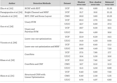
Based on the results reported, it can be inferred from Table 11 that shadow detection by using Structured Convolutional Neural Network with linear optimiza-tion proposed by Shen et al. [31] outperforms all other techniques for the three datasets, namely, UIUC, UCF, and CMU. While the learning techniques deployed by feature based methods and region based methods provide good detection results, the time and memory consumption are higher for these methods.

Zhu et al. [41] mentioned that their method consumed approximately 9GB for training 125 images of average size, 480×320. The automatic feature learning pro-posed by Khan et al. [19] requires ∼1GB memory and ~1 hour for training each of the above mentioned data-bases. The selection of the training images also con-tributes to the efficiency of detection algorithm.

6. Conclusion

Shadows are a natural phenomenon that appears on a surface due to obstruction of light by an object. Since their presence may cause complications in image vision applications, the detection and elimination of shadows have become an important topic of research. Shadow detection and removal is considered as an image en-hancement technique and is therefore included in such pre-processing stage of computer vision applications as object detection and video examination. This makes it necessary to develop techniques that can detect and re-move shadows accurately in very limited time.

(15)

tech-89

Table 11

A quantitative analysis of shadow detection methods

Author Detection Methods Dataset _{error rate}Shadow Non- shadow _{error rate} _{error rate}Balanced

Zhu et al. [41] BCRF with BDT UCF 36.1 6.60 21.35

Panagopoulos et al. [24] Bright Channel and MRF UCF 31.7 10.6 21.15

Lalonde et al. [20] BDT, CRF and Scene Layout CMU 26.9 3.60 15.25

Guo et al. [16]

Unary SVM UCF 63.3 2.70 33.0

UIUC 45.7 8.90 27.3

Unary and Pairwise SVM

UCF 26.7 6.30 16.5

UIUC 28.4 4.80 16.6

Vicente et al. [36]

Leave-one-out optimization UCF 22.9 6.20 14.5

UIUC 14.9 4.20 9.50

Leave-one-out optimization and MRF UCF 20.0 6.40 13.2

UIUC 9.90 4.40 7.20

Khan et al. [19]

ConvNets UCF 27.5 7.90 17.7

UIUC 16.4 5.30 10.6

ConvNets and CRF

UCF 22.0 7.40 14.7

CMU 16.7 9.10 12.9

UIUC 15.3 4.50 9.90

Shen et al. [31] Structured CNN with_{Linear Optimization}

UCF 8.40 6.60 7.50

CMU 8.40 2.30 5.35

UIUC 8.70 4.97 6.83

*The values were derived/taken from the papers discussed in this review

niques were classified under five categories, namely, invariant based detection, featubased detection, re-gion-based detection, color model based detection and interactive shadow detection. A qualitative and quanti-tative comparison is also included. The major observa-tions made out of the survey may be stated as follows:

1 Even though the invariant-based shadow detection

techniques provide results faster, the algorithms require prior knowledge of illuminant direction and high quality input images. Further, the results depend on the edge detection algorithm employed for generating edgemap.

2 Feature-based techniques provide better results

with optimal feature set when compared to in-variant based approach. However, the algorithms demand high computational and memory

require-ments to train the classifier for detection.

3 Region-based shadow detection algorithms,

al-though provide better results, demand higher computational requirements as the algorithms are based on learned features. Simple and fast color model based algorithms very often wrongly classi-fy dark regions as shadows. Moreover, interactive shadow detection process, though appears to be simpler than automatic techniques, is not conve-nient for the user in case of multiple shadow re-gions. Soft shadows that span multiple surfaces also pose challenge in accurate detection of shad-ows.

4 Another major observation is that the accuracy of

(16)

interac-tions are also considered. A single shadow might have different regions in it- the dark umbra region and the lighter penumbra region. An efficient de-tection algorithm must be capable of locating both

the regions. Detection of self-shadows and heavily scattered shadows are also challenging. The risk of misclassifying dark objects as shadows should also be addressed.

References

1. Al-Najdawi, N., Bez, H. E., Singhai, J., Edirisinghe, E. A. A Survey of Cast Shadow Detection Algorithms. Pattern Recognition Letters, 2012, 33(6), 752–764. http://doi. org/10.1016/j.patrec.201 1.12.013.

2. Arbel, E., Hel-Or, H. Shadow Removal Using Intensity Surfaces and Texture Anchor Points. IEEE Transactions on Pattern Analysis and Machine Intelligence, 2011, 33(6), 1202–1216. https://doi.org/10.1109/TPAMI.2010.157 3. Barrow, H. G., Tenenbaum, J. M. Recovering Intrinsic

Scene Characteristics from Images. Computer Vision Systems, 1978, 3–26.

4. Cucchiara, R., Grana, C., Piccardi, M., Prati, A. Detect-ing MovDetect-ing Objects, Ghosts, and Shadows in Video Streams. IEEE Transactions on Pattern Analysis and Machine Intelligence, 2003, 25(10), 1337–1342. http:// doi.org/10.1109/TPAMI.2003.1233 909.

5. Dong, Q., Liu, Y., Zhao, Q., Yang, H. Detecting Soft Shad-ows in a Single Outdoor Image: from Local Edge-Based Models to Global Constraints. Computers and Graph-ics, 2014, 38(1), 310–319. https://doi.org/10.1016/j. cag.2013.11.005

6. Figov, Z., Tal, Y., Koppel, M. Detecting and Removing Shadows. Proceedings of 7th IASTED International Conference on Computer Graphics and Imaging, 2004. 7. Finlayson, G. D., Drew, M. S., Lu, C. Entropy

Minimi-zation for Shadow Removal. International Journal of Computer Vision, 2009, 85(1), 35–57. https://doi. org/10.1007/s11263-009-0243-z

8. Finlayson, G. D., Hordley, S. D. Color Constancy at a Pix-el. Journal of the Optical Society of America, 2001, 18(2), 253–264. http://doi.org/10.1364/JOSAA .18.000253 9. Finlayson, G. D., Hordley, S. D., Drew, M. S. Removing

Shadows from Images. Proceedings of the 7th Euro-pean Conference on Computer Vision, 2002, 823–836. https://doi.org/10.1007/3-540-47979-1_55

10. Finlayson, G. D., Hordley, S. D., Lu, C., Drew, M. S. On the Removal of Shadows from Images. IEEE Transactions on Pattern Analysis and Machine Intelligence, 2006,

28(1), 59–68. https://doi.org/10.1109/TPAMI.2006.18 11. Gevers, T., Stokman, H. Classifying Color Edges in

Vid-eo into Shadow-GVid-eometry, Highlight, or Material Tran-sitions. IEEE Transactions on Multimedia, 2003, 5(2), 237–243. https://doi.org/10.1109/TMM.2003.811620 12. Gijsenij, A., Gevers, T. Shadow Edge Detection Using

Geometric and Photometric Features. Proceedings of the 16th IEEE International Conference on Image Pro-cessing (ICIP), Cairo, Egypt, Nov 7-10, 2009, 693–696. http://doi.org/10.1 109/ICIP.2009.5414089

13. Golchin, M., Khalid, F., Abdullah, L. N., Davarpanah, S. H. Shadow Detection Using Color and Edge Informa-tion. Journal of Computer Science, 2013, 9(11), 1575– 1588. https://doi.org/10.3844/jcssp.2013.1575.1588 14. Gong, H., Cosker, D. P. Interactive Shadow Removal and

Ground Truth for Variable Scene Categories. Proceed-ings of the British Machine Vision Conference, 2014. http://dx.doi.org/10.5244 /C.28.36

15. Gong, H., Cosker, D., Li, C., Brown, M. User-Aided Sin-gle Image Shadow Removal. Proceedings of the IEEE International Conference on Multimedia and Expo(IC-ME), San Jose, CA, USA, July 15-19, 2013, 1–6. https:// doi.org/10.1109/ICME.2013.6607463

16. Guo, R., Dai, Q., Hoiem, D. Paired Regions for Shadow Detection and Removal. IEEE Transactions on Pattern Analysis and Machine Intelligence, 2013, 35(12), 2956– 2967. http://doi.org/10.1109/TPA MI.2012.214

17. He, Q., Chu, C.-H. H. A New Shadow Removal Method for Color Images. Advances in Remote Sensing, 2013, 77–84. http://doi.org/10.4236/ars.2 013.22011

18. Jiang, X., Schofield, A., Wyatt, J. Shadow Detection Based on Colour Segmentation and Estimated Illumi-nation. Proceedings of the British Machine Vision Con-ference, 2011, 1-11. http://doi.org/10.52 44 /C.25.87 19. Khan, S. H., Bennamoun, M., Sohel, F., Togneri, R.

(17)

91

org/10.1109/TPAMI.2015.2462 355

20. Lalonde, J. F., Efros, A. A., Narasimhan, S. G. Detecting Ground Shadows in Outdoor Consumer Photographs. In: Daniilidis K., et al. (Eds.), European Conference on Computer Vision, Lecture Notes in Computer Sci-ence, 6312. Springer, Berlin-Heidelberg, 322–335, 2010. http://d oi.org/10.1007/978-3-642-15552-9_24

21. Lu, C., Drew, M. S. Shadow Segmentation and Shad-ow-Free Chromaticity via Markov Random Fields. In: Color Imaging Conference, IS&T – The Society for Im-aging Science and Technology, 2005, 2005(1), 125–129. 22. Murali, S., Govindan, V. K. Shadow Detection and

Re-moval from a Single Image Using LAB Color Space. Cy-bernetics and Information Technologies, 2013, 13(1), 95–103. https://doi.org/10.2478/cait-2013-0009 23. Nielsen, M., Madsen, C.B. Graph Cut Based

Segmen-tation of Soft Shadows for Seamless Removal and Augmentation. In: Ersbøll, B.K., Pedersen, K. S. (Eds.), Scandinavian Conference on Image Analysis, Lecture Notes in Computer Science, 4522, Springer, Berlin-Hei-delberg, 918–927, 2007. https://doi.org/10.1007/978-3-540-73040-8_93

24. Panagopoulos, A., Wang, C., Samaras, D., Paragios, N. Estimating Shadows with the Bright Channel Cue. In: Kutulakos K. N. (Eds.) Trends and Topics in Computer Vision, ECCV 2010, Lecture Notes in Computer Sci-ence, 6554, Springer, Berlin-Heidelberg, 1-12, 2010. https://doi.org/10.1007/978-3-642-35740-4_1

25. Salvador, E., Cavallaro, A., Ebrahimi, T. Shadow Identi-fication and ClassiIdenti-fication Using Invariant Color Mod-els. Proceedings of IEEE International Conference on Acoustics, Speech, and Signal Processing, Salt Lake City, USA, 7-11 May, 2001, 3, 1545–1548. http://doi. org/10.1109/ICASSP.2001.941 227

26. Salvador, E., Cavallaro, A., Ebrahimi, T. Cast Shadow Segmentation Using Invariant Color Features. Com-puter Vision and Image Understanding, 2004, 95(2), 238–259. http://doi.or g/10.1016/j.cviu.2004.03.008 27. Sanin, A., Sanderson, C., Lovell, B. C. Shadow

detec-tion: A Survey and Comparative Evaluation of Recent Methods. Pattern Recognition, 2012, 45(4), 1684–1695. http://doi.org/10.1016/j.patcog.2011.10.0 01

28. Sasi, R. K., Govindan, V. K. Fuzzy Split and Merge for Shadow Detection. Egyptian Informatics Journal, 2014, 16(1), 29–35. http://doi.org/10.1016/ j.eij.2014.11.003 29. Sasi, R. K., Govindan, V. K. Shadow Detection and

Re-moval from Real Images: State of Art. Proceedings of the 3rd International Symposium on Women in

Comput-ing and Informatics, Kochi, India, August 10 - 13, 2015, 309–317. http://doi.org/10.1 145/2791405.2791450 30. Serra, M., Penacchio, O., Benavente, R., Vanrell, M.

Names and Shades of Color for Intrinsic Image Estima-tion. Proceedings of the IEEE Computer Society Con-ference on Computer Vision and Pattern Recognition, Providence, RI, USA, June 16-21, 2012, 278–285. http:// doi.org/10.1109/CVPR.201 2.6247686

31. Shen, L., Chua, T. W., Leman, K. Shadow Optimization from Structured Deep Edge Detection. Proceedings of the IEEE Computer Society Conference on Com-puter Vision and Pattern Recognition, Boston, USA, June 07–12, 2015, 2067–2074. https://doi.org/10.1109/ CVPR.2015.7298818

32. Shor, Y., Lischinski, D. The Shadow Meets the Mask: Pyramid-Based Shadow Removal. Computer Graphics Forum, 2008, 27(2), 577–586. https://doi.org/10.1111/ j.1467-8659.2008.01155.x

33. Tian, J., Qi, X., Qu, L., Tang, Y. New Spectrum Ratio Properties and Features for Shadow Detection. Pattern Recognition, 2016, 51, 85–96. https://doi.org/10.1016/j. patcog.2015.09.006

34. Tian, J., Sun, J., Tang, Y. Tricolor Attenuation Mod-el for Shadow Detection. IEEE Transactions on Im-age Processing, 2009, 18(10), 2355–2363. http://d oi.org/10.1109/TIP.2009.2026682

35. Vicente, T. F. Y., Yu, C.P., Samaras, D. Single Image Shad-ow Detection Using Multiple Cues in a Supermodular MRF. British Machine Vision Conference, 2013, 1–12. http://doi.org/10.524 4/C.27.126

36. Vicente, T. F. Y., Hoai, M., Samaras, D. Leave-One-Out Kernel Optimization for Shadow Detection. Proceed-ings of the IEEE International Conference on Comput-er Vision, Santiago, Chile, Dec 7–13, 2015, 3388–3396. http://doi.org/10.1109/ICCV.201 5.387

37. Wu, Q., Zhang, W., Vijaya Kumar, B. V. K. Strong Shad-ow Removal via Patch-Based ShadShad-ow Edge Detec-tion. Proceedings of IEEE International Conference on Robotics and Automation, Saint Paul, MN, USA, May 14-18, 2012, 2177–2182. https://doi.org/10.1109/ ICRA.2012.6224561

38. Wu, T. P., Tang, C. K. A Bayesian Approach for Shad-ow Extraction from a Single Image. Proceedings of the IEEE International Conference on Computer Vision, Beijing, China, Oct 17-21, 2005, 1, 480–487. http://doi. org/10.1109/ICCV.2 005.4