Electromagnetic ﬁeld vulnerability of complex systems – an application of EM topology

(1)

Adv. Radio Sci., 6, 273–277, 2008 www.adv-radio-sci.net/6/273/2008/

Advances in

Radio Science

Electromagnetic field vulnerability of complex systems – an

application of EM topology

R. Kanyou Nana1, S. Dickmann1, and F. Sabath2

1_{Helmut-Schmidt-Universität/Universität der Bundeswehr Hamburg, Fakultät für Elektrotechnik, Hamburg, Germany} 2_{Wehrwissenschaftliches Institut für Schutztechnologien–ABC Schutz, Munster, Germany}

Abstract. In complex systems like ships or airplanes many tasks vital to the function of the system are executed by electronic equipment. Earlier research Camp (2004)– Nitsch (2005) has shown that there are frequency ranges in many of these systems, in which disturbances in the sys-tem will be observed if an external electromagnetic field ex-ceeds a certain amplitude limit. On the basis of a simpli-fied model in which the dominating coupling mechanisms in complex systems are shown, we will present a method which allows to analyze the vulnerability to electromagnetic fields. The method is based on the segmentation of the initial prob-lem into subprobprob-lems with respect to the coupling mecha-nisms. Under the assumption that the obtained classes can be handled separately, the subproblems are solved and super-posed to the overall solution. The Electromagnetic Topology Baum (1982)–Lee (1982) is used to solve the subproblems. This leads to a hybrid method combining different solution approaches. The subproblems are decomposed into smaller subproblems with respect to the shielding levels. This pro-cedure allows us to determine the coupled disturbances into the system. Finally the solution is verified with respect to prescripted limits.

1 Introduction

Complex systems comprise a considerable amount of electric and electronic devices, which contain COTS (commercial-of-the-shelf)-components. In many of these systems fre-quency ranges exist in which disturbances in the sys-tem can be observed starting from a particular magnitude Camp (2004)–Nitsch (2005). In the case that the spectra of electromagnetic fields (EM-fields) produced by impulse gen-erators are within those frequency ranges, the vulnerability of such systems to EM-fields must be evaluated. A methodol-ogy will be applied which allows us to identify the critical coupling paths of a system during an electromagnetic attack.

Correspondence to: R. Kanyou Nana

([email protected]) Date: 1 February 2008

Electromagnetic field vulnerability of complex systems – an

application of EM topology

R. Kanyou Nana1_{, S. Dickmann}1_{, and F. Sabath}2

1_{Helmut–Schmidt–Universität / Universität der Bundeswehr Hamburg, Fakultät für Elektrotechnik} 2_{Wehrwissenschaftliches Institut für Schutztechnologien–ABC Schutz, Munster}

Abstract.In complex systems like ships or airplanes many tasks vital to the function of the system are executed by electronic equipment. Earlier research [1]–[3] has shown that there are frequency ranges in many of these systems, in which disturbances in the system will be observed if an exter-nal electromagnetic field exceeds a certain amplitude limit. On the basis of a simplified model in which the dominating coupling mechanisms in complex systems are shown, we will present a method which allows to analyze the vulnerability to electromagnetic fields. The method is based on the segmen-tation of the initial problem into subproblems with respect to the coupling mechanisms. Under the assumption that the ob-tained classes can be handled separately, the subproblems are solved and superposed to the overall solution. The Electro-magnetic Topology [4]–[5] is used to solve the subproblems. This leads to a hybrid method combining different solution approaches. The subproblems are decomposed into smaller subproblems with respect to the shielding levels. This pro-cedure allows us to determine the coupled disturbances into the system. Finally the solution is verified with respect to prescripted limits.

1 Introduction

Complex systems comprise a considerable amount of electric and electronic devices, which contain COTS (commercial-of-the-shelf)-components. In many of these systems fre-quency ranges exist in which disturbances in the system can be observed starting from a particular magnitude [1]–[3]. In the case that the spectra of electromagnetic fields (EM-fields) produced by impulse generators are within those frequency ranges, the vulnerability of such systems to EM-fields must be evaluated. A methodology will be applied which allows Correspondence to:R. Kanyou Nana

([email protected])

us to identify the critical coupling paths of a system during an electromagnetic attack.

2 Analysis of the problem

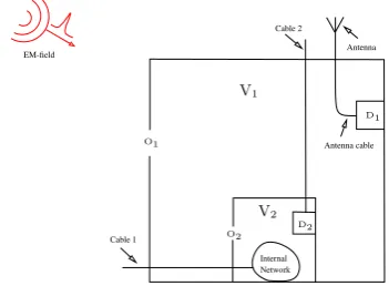
The model of the considered system is shown in Figure1. The system consists of two volumesV1andV2with the

cor-responding aperturesO1andO2. Within the volumeV1, the

volumeV2and the deviceD1are located.D1is connected

to an external antenna via an antenna cable. The volumeV2

EM-field

Internal Network

D2 D1

Cable 1

Cable 2 Antenna

O1

O2

Antenna cable

V1

V2

Fig. 1.Geometry of the system illuminated by an EM-field

contains the internal network to be analysed, as well as the deviceD2. Both of them are connected to the outside world

via separate cables. The entire system is illuminated by an EM-Field.

In order to clarify the dominating interaction mechanisms in complex systems, i.e. aperture coupling, conductive coup-ling, radiation of cables, the following assumptions are made:

Fig. 1. Geometry of the system illuminated by an EM-field.

2 Analysis of the problem

The model of the considered system is shown in Fig. 1. The system consists of two volumes V1 and V2 with the

corre-sponding apertures O1 and O2. Within the volume V1, the

volume V2and the device D1are located. D1is connected

to an external antenna via an antenna cable. The volume V2contains the internal network to be analysed, as well as

the device D2. Both of them are connected to the outside

world via separate cables. The entire system is illuminated by an EM-Field. In order to clarify the dominating interac-tion mechanisms in complex systems, i.e. aperture coupling, conductive coupling, radiation of cables, the following as-sumptions are made:

– the antenna cable radiates (bad shielding, low symmetry of the antenna or insufficient balun at the antenna), – cable 2 radiates only within the volume 2 (no shielding), – cable 1 does not radiate (ideal shielding of the cable 1

in both volumes 1 and 2).

Figure 2 shows the coupling model corresponding to Fig. 1, which is used for evaluation of the internal network in vol-ume 2, taking into account all intermediate results.

(2)

274 R. Kanyou Nana et al.: Vulnerability analysis of complex systems

–the antenna cable radiates (bad shielding, low symmetry of the antenna or insufficient balun at the antenna), –cable 2 radiates only within the volume 2 (no shielding), –cable 1 does not radiate (ideal shielding of the cable 1

in both volumes 1 and 2).

Figure2shows the coupling model corresponding to Figu-re1, which is used for evaluation of the internal network in volume 2, taking into account all intermediate results. Consequently the coupling paths in the subvolumes can be

Internal Network

D2 D1

I3

I2 I1

V1

V2

Fig. 2.Coupling paths in the subvolumes

described:

–the internal field in the volume 1 is caused by the pre-sence of the aperture 1 and the radiating antenna cable, –the internal field in the volume 2 is generated by the ra-diation of the aperture 2 and the radiating part of cable 2 in volume 2.

If the EM-fields of the complete system were calculated us-ing a numerical solver, it could be observed that the solution depends on several coupling mechanisms. But the influence of a single mechanism can’t be investigated separately in this way. In addition, this solution method requires a completely new calculation of the problem for any change in the sys-tem. In order to eliminate these disadvantages we propose the following modifications of the solution method: The ini-tial problem will be solved based on the solutions of the sub-problems. Therefore the subproblems must be classified (see Figure3). If the initial problem

1. can be reduced to these subproblems, 2. these subproblems can be solved, and

3. all solutions can be combined at the component-level, then the vulnerability analysis of the internal network under an external electromagnetic attack is possible.

3 Methodology for the vulnerability analysis

The methodology explained in this chapter, in order to as-sess the vulnerability of a system to electromagnetic attacks, is primarily based on the decomposition of the whole pro-blem into subpropro-blems (classes) with respect to the coupling mechanism. For this segmentation a detailed knowledge of the system is required. This, for example, can be acquired by geometrical analysis or by precise measurement of the transfer functions of the system. The main objective of this decomposition is to allow a separate solution of the resulting subproblems. As a consequence, a change in the structure of the system (e.g. addition of new coupling paths or re-moval of nonrelevant coupling paths) does not necessarily require a change of the whole solution approach. Therefore it is possible to reuse the old results in further computations. Figure3illustrates the segmentation of the original problem into subproblems with reference to the first shielding level. The classification of the subproblems is as follows:

1 2

3 4

∼

=

1 2 3 4

Int.N

+

Int.N

+ Int.N+

Int.N Int.N

Fig. 3.Decomposition of the initial problem into subproblems

1. radiation of a cable into a subvolume,

2. direct radiation of a cable into the internal network, 3. direct coupling to the internal network through a

con-nected wire,

4. coupling through apertures.

The solution of the generated classes allows an identification of the significant and nonrelevant coupling paths. Thus, it is possible to simplify the simulation of the complete system by omitting the nonrelevant coupling mechanisms. After the segmentation of the problem, the subproblems will

Fig. 2. Coupling paths in the subvolumes.

Consequently the coupling paths in the subvolumes can be described:

– the internal field in the volume 1 is caused by the pre-sence of the aperture 1 and the radiating antenna cable, – the internal field in the volume 2 is generated by the ra-diation of the aperture 2 and the radiating part of cable 2 in volume 2.

If the EM-fields of the complete system were calculated us-ing a numerical solver, it could be observed that the solution depends on several coupling mechanisms. But the influence of a single mechanism can’t be investigated separately in this way. In addition, this solution method requires a completely new calculation of the problem for any change in the sys-tem. In order to eliminate these disadvantages we propose the following modifications of the solution method: The ini-tial problem will be solved based on the solutions of the sub-problems. Therefore the subproblems must be classified (see Fig. 3). If the initial problem

1. can be reduced to these subproblems, 2. these subproblems can be solved, and

3. all solutions can be combined at the component-level, then the vulnerability analysis of the internal network under an external electromagnetic attack is possible.

3 Methodology for the vulnerability analysis

The methodology explained in this chapter, in order to as-sess the vulnerability of a system to electromagnetic attacks, is primarily based on the decomposition of the whole pro-blem into subpropro-blems (classes) with respect to the coupling mechanism. For this segmentation a detailed knowledge of the system is required. This, for example, can be acquired by geometrical analysis or by precise measurement of the

– the antenna cable radiates (bad shielding, low symmetry of the antenna or insufficient balun at the antenna),

– cable 2 radiates only within the volume 2 (no shielding),

– cable 1 does not radiate (ideal shielding of the cable 1 in both volumes 1 and 2).

Figure2shows the coupling model corresponding to Figu-re 1, which is used for evaluation of the internal network in volume 2, taking into account all intermediate results. Consequently the coupling paths in the subvolumes can be

Internal Network

D2

D1

I3

I2 I1

V1

V2

Fig. 2.Coupling paths in the subvolumes

described:

– the internal field in the volume 1 is caused by the pre-sence of the aperture 1 and the radiating antenna cable,

– the internal field in the volume 2 is generated by the ra-diation of the aperture 2 and the radiating part of cable 2 in volume 2.

If the EM-fields of the complete system were calculated us-ing a numerical solver, it could be observed that the solution depends on several coupling mechanisms. But the influence of a single mechanism can’t be investigated separately in this way. In addition, this solution method requires a completely new calculation of the problem for any change in the sys-tem. In order to eliminate these disadvantages we propose the following modifications of the solution method: The ini-tial problem will be solved based on the solutions of the sub-problems. Therefore the subproblems must be classified (see Figure3). If the initial problem

1. can be reduced to these subproblems,

2. these subproblems can be solved, and

3. all solutions can be combined at the component-level,

then the vulnerability analysis of the internal network under an external electromagnetic attack is possible.

3 Methodology for the vulnerability analysis

The methodology explained in this chapter, in order to as-sess the vulnerability of a system to electromagnetic attacks, is primarily based on the decomposition of the whole pro-blem into subpropro-blems (classes) with respect to the coupling mechanism. For this segmentation a detailed knowledge of the system is required. This, for example, can be acquired by geometrical analysis or by precise measurement of the transfer functions of the system. The main objective of this decomposition is to allow a separate solution of the resulting subproblems. As a consequence, a change in the structure of the system (e.g. addition of new coupling paths or re-moval of nonrelevant coupling paths) does not necessarily require a change of the whole solution approach. Therefore it is possible to reuse the old results in further computations. Figure3illustrates the segmentation of the original problem into subproblems with reference to the first shielding level. The classification of the subproblems is as follows:

1 2

3 4

∼

=

1 2 3 4

Int.N

+

Int.N

+ Int.N +

Int.N Int.N

Fig. 3.Decomposition of the initial problem into subproblems

1. radiation of a cable into a subvolume,

2. direct radiation of a cable into the internal network,

3. direct coupling to the internal network through a con-nected wire,

The solution of the generated classes allows an identification of the significant and nonrelevant coupling paths. Thus, it is possible to simplify the simulation of the complete system by omitting the nonrelevant coupling mechanisms.

After the segmentation of the problem, the subproblems will

Fig. 3. Decomposition of the initial problem into subproblems. be solved separately or treated in subgroups with the help of the Electromagnetic Topology (EMT). The significant results of these intermediate steps are the internal EM-fields due to the respective mechanisms as well as the external equivalent sources. Both are used for the excitation of the internal net-work on the basis of equivalent generators along the cables and wires (tubes) or as lumped sources at the gates of the de-vices or terminals (junctions). With knowledge of the equi-valent sources, the propagation behavior of the waves along thetubesas well as the scattering behavior of the connected devices is described with the BLT (Baum, Liu, Tesche)-equation [6]–[7]. The BLT-Tesche)-equation was firstly implemented by Tesche and Liu in the QV7TA code [8]. More recent work resulted in the CRIPTE software package [9]–[10]. The main advantage using EMT for the vulnerability analysis of com-plex systems to EM-Fields is that results of different solution approachs (e.g. measurements and numerical simulations or a combination of different kinds of simulations like FDTD and CRIPTE) can be combined. Thus, for each subproblem the most efficient method can be chosen.

After the solution of the subproblems their results will be su-perposed to obtain the general solution. In the last step this will allow an assessment of the vulnerability of the system. This general solution will finally be compared to the pres-cripted limits from the standards [11]. When the obtained ge-neral solution for a specific EM-field generator is below the prescripted limits the system will be considered as non vul-nerable against electromagnetic fields produced by this field generator. Otherwise, it is considered as vulnerable.

4 Handling of the wire’s coupling on one shielding level

In the case of a connection of an external antenna with an internal cable as well as in the case of a cable feedthrough on one shielding level, the delimitation of a volume is not rea-lisable when using the EMT. The use of equivalent current sources is helpful in this situation. For the example of the previously explained first class, Figure4 demonstrates the described situation. The deviceD1 has been replaced by its

input impedanceZ. In this approach the antenna is replaced

∼

=

I₁

Z Z

Fig. 4. Replacement of the antenna current with one equivalent current source

by a current sourceI1which generates the antenna current at

its foot point. The currentI1 is determined as follows: The

impedance Z1 of the device D1 including the cable within

V1 is determined as seen from the antenna foot point. This

is done through the definition of a fictitious internal current sourceIthat replaces the excited external antenna (see Figu-re5). Its input impedance represents the impedanceZ1. Now

I

Z

Fig. 5. Placement of one fictitious current source in order to com-pute the impedance at the low end of the antenna

the equivalent currentI1 can be calculated. By doing this,

the above-mentioned network (antenna cable +Z) is replaced through the previously determined (input) impedanceZ1(see

Figure6).

I1

Z₁

Fig. 6. Replacement of the network (antenna cable +Z) withZ1in

order to compute the equivalent current sourceI1

5 Validation of the method

5.1 Geometry of the considered system

The following laboratory set-up has been examined for the validation of the method described above.

x y

z

R UR

− →

k

− →

E

− →

H

Fig. 7.Laboratory set-up for the validation of the method

Fig. 4. Replacement of the antenna current with one equivalent

current source.

transfer functions of the system. The main objective of this decomposition is to allow a separate solution of the resulting subproblems. As a consequence, a change in the structure of the system (e.g. addition of new coupling paths or removal of nonrelevant coupling paths) does not necessarily require a change of the whole solution approach. Therefore it is possi-ble to reuse the old results in further computations. Figure 3 illustrates the segmentation of the original problem into sub-problems with reference to the first shielding level.

The classification of the subproblems is as follows: 1. radiation of a cable into a subvolume,

2. direct radiation of a cable into the internal network, 3. direct coupling to the internal network through a

con-nected wire,

The solution of the generated classes allows an identification of the significant and nonrelevant coupling paths. Thus, it is possible to simplify the simulation of the complete sys-tem by omitting the nonrelevant coupling mechanisms. Af-ter the segmentation of the problem, the subproblems will be solved separately or treated in subgroups with the help of the Electromagnetic Topology (EMT). The significant re-sults of these intermediate steps are the internal EM-fields

(3)

R. Kanyou Nana et al.: Vulnerability analysis of complex systems 275

R. Kanyou Nana et al.: Vulnerability analysis of complex systems

3 be solved separately or treated in subgroups with the help of

the Electromagnetic Topology (EMT). The significant results

of these intermediate steps are the internal EM-fields due to

the respective mechanisms as well as the external equivalent

sources. Both are used for the excitation of the internal

net-work on the basis of equivalent generators along the cables

and wires (

tubes

) or as lumped sources at the gates of the

de-vices or terminals (

junctions

). With knowledge of the

equi-valent sources, the propagation behavior of the waves along

the

tubes

as well as the scattering behavior of the connected

devices is described with the BLT (Baum, Liu,

Tesche)-equation [6]–[7]. The BLT-Tesche)-equation was firstly implemented

by Tesche and Liu in the QV7TA code [8]. More recent work

resulted in the CRIPTE software package [9]–[10]. The main

advantage using EMT for the vulnerability analysis of

com-plex systems to EM-Fields is that results of different solution

approachs (e.g. measurements and numerical simulations or

a combination of different kinds of simulations like FDTD

and CRIPTE) can be combined. Thus, for each subproblem

the most efficient method can be chosen.

After the solution of the subproblems their results will be

su-perposed to obtain the general solution. In the last step this

will allow an assessment of the vulnerability of the system.

This general solution will finally be compared to the

pres-cripted limits from the standards [11]. When the obtained

ge-neral solution for a specific EM-field generator is below the

prescripted limits the system will be considered as non

vul-nerable against electromagnetic fields produced by this field

generator. Otherwise, it is considered as vulnerable.

4 Handling of the wire’s coupling on one shielding level

In the case of a connection of an external antenna with an

internal cable as well as in the case of a cable feedthrough on

one shielding level, the delimitation of a volume is not

rea-lisable when using the EMT. The use of equivalent current

sources is helpful in this situation. For the example of the

previously explained first class, Figure

4 demonstrates the

described situation. The device

D

1

has been replaced by its

input impedance

Z

. In this approach the antenna is replaced

∼

=

I₁

Z Z

Fig. 4.

Replacement of the antenna current with one equivalent

current source

by a current source

I

1

which generates the antenna current at

its foot point. The current

I

1

is determined as follows: The

impedance

Z

1

of the device

D

1

including the cable within

V

1

is determined as seen from the antenna foot point. This

is done through the definition of a fictitious internal current

source

I

that replaces the excited external antenna (see

Figu-re

5 ). Its input impedance represents the impedance

Z

1

. Now

I

Z

Fig. 5.

Placement of one fictitious current source in order to

com-pute the impedance at the low end of the antenna

the equivalent current

I

1

can be calculated. By doing this,

the above-mentioned network (antenna cable +

Z

) is replaced

through the previously determined (input) impedance

Z

1

(see

Figure

6 ).

I₁ Z₁

Fig. 6.

Replacement of the network (antenna cable +

Z

) with

Z

1

in

order to compute the equivalent current source

I

1

5 Validation of the method

5.1 Geometry of the considered system

The following laboratory set-up has been examined for the

validation of the method described above.

x y

z

R UR

− →

k

− →

E

− →

H

Fig. 7.

Laboratory set-up for the validation of the method

Fig. 5. Placement of one fictitious current source in order to

com-pute the impedance at the low end of the antenna.

R. Kanyou Nana et al.: Vulnerability analysis of complex systems

3 be solved separately or treated in subgroups with the help of

the Electromagnetic Topology (EMT). The significant results

of these intermediate steps are the internal EM-fields due to

the respective mechanisms as well as the external equivalent

sources. Both are used for the excitation of the internal

net-work on the basis of equivalent generators along the cables

and wires (

tubes

) or as lumped sources at the gates of the

de-vices or terminals (

junctions

). With knowledge of the

equi-valent sources, the propagation behavior of the waves along

the

tubes

as well as the scattering behavior of the connected

devices is described with the BLT (Baum, Liu,

Tesche)-equation [6]–[7]. The BLT-Tesche)-equation was firstly implemented

by Tesche and Liu in the QV7TA code [8]. More recent work

resulted in the CRIPTE software package [9]–[10]. The main

advantage using EMT for the vulnerability analysis of

com-plex systems to EM-Fields is that results of different solution

approachs (e.g. measurements and numerical simulations or

a combination of different kinds of simulations like FDTD

and CRIPTE) can be combined. Thus, for each subproblem

the most efficient method can be chosen.

After the solution of the subproblems their results will be

su-perposed to obtain the general solution. In the last step this

will allow an assessment of the vulnerability of the system.

This general solution will finally be compared to the

pres-cripted limits from the standards [11]. When the obtained

ge-neral solution for a specific EM-field generator is below the

prescripted limits the system will be considered as non

vul-nerable against electromagnetic fields produced by this field

generator. Otherwise, it is considered as vulnerable.

4 Handling of the wire’s coupling on one shielding level

In the case of a connection of an external antenna with an

internal cable as well as in the case of a cable feedthrough on

one shielding level, the delimitation of a volume is not

rea-lisable when using the EMT. The use of equivalent current

sources is helpful in this situation. For the example of the

previously explained first class, Figure

4 demonstrates the

described situation. The device

D

1

has been replaced by its

input impedance

Z

. In this approach the antenna is replaced

∼

=

I₁

Z Z

Fig. 4.

Replacement of the antenna current with one equivalent

current source

by a current source

I

1

which generates the antenna current at

its foot point. The current

I

1

is determined as follows: The

impedance

Z

1

of the device

D

1

including the cable within

V

1

is determined as seen from the antenna foot point. This

is done through the definition of a fictitious internal current

source

I

that replaces the excited external antenna (see

Figu-re

5 ). Its input impedance represents the impedance

Z

1

. Now

I

Z

Fig. 5.

Placement of one fictitious current source in order to

com-pute the impedance at the low end of the antenna

the equivalent current

I

1

can be calculated. By doing this,

the above-mentioned network (antenna cable +

Z

) is replaced

through the previously determined (input) impedance

Z

1

(see

Figure

6 ).

I₁ Z₁

Fig. 6.

Replacement of the network (antenna cable +

Z

) with

Z

1

in

order to compute the equivalent current source

I

1

5 Validation of the method

5.1 Geometry of the considered system

The following laboratory set-up has been examined for the

validation of the method described above.

x y

z

R UR

− →

k − →

E

− → H

Fig. 7.

Laboratory set-up for the validation of the method

Fig. 6. Replacement of the network (antenna cable + Z) with Z1in

order to compute the equivalent current source.I1

due to the respective mechanisms as well as the external equivalent sources. Both are used for the excitation of the internal network on the basis of equivalent generators along the cables and wires (tubes) or as lumped sources at the gates of the devices or terminals (junctions). With knowledge of the equivalent sources, the propagation be-havior of the waves along the tubes as well as the scat-tering behavior of the connected devices is described with the BLT (Baum, Liu, Tesche)-equation Tesche et al. (1996)– Paul (1994). The BLT-equation was firstly implemented by Tesche and Liu in the QV7TA code Tesche and Liu (1978). More recent work resulted in the CRIPTE software package ESI/ONERA (2003)–Parmantier et al. (1993). The main ad-vantage using EMT for the vulnerability analysis of complex systems to EM-Fields is that results of different solution ap-proachs (e.g. measurements and numerical simulations or a combination of different kinds of simulations like FDTD and CRIPTE) can be combined. Thus, for each subproblem the most efficient method can be chosen.

After the solution of the subproblems their results will be su-perposed to obtain the general solution. In the last step this will allow an assessment of the vulnerability of the system. This general solution will finally be compared to the pres-cripted limits from the standards Steinmetz (2006). When the obtained general solution for a specific EM-field generator is below the prescripted limits the system will be considered be solved separately or treated in subgroups with the help of the Electromagnetic Topology (EMT). The significant results of these intermediate steps are the internal EM-fields due to the respective mechanisms as well as the external equivalent sources. Both are used for the excitation of the internal net-work on the basis of equivalent generators along the cables and wires (tubes) or as lumped sources at the gates of the de-vices or terminals (junctions). With knowledge of the equi-valent sources, the propagation behavior of the waves along thetubesas well as the scattering behavior of the connected devices is described with the BLT (Baum, Liu, Tesche)-equation [6]–[7]. The BLT-Tesche)-equation was firstly implemented by Tesche and Liu in the QV7TA code [8]. More recent work resulted in the CRIPTE software package [9]–[10]. The main advantage using EMT for the vulnerability analysis of com-plex systems to EM-Fields is that results of different solution approachs (e.g. measurements and numerical simulations or a combination of different kinds of simulations like FDTD and CRIPTE) can be combined. Thus, for each subproblem the most efficient method can be chosen.

After the solution of the subproblems their results will be su-perposed to obtain the general solution. In the last step this will allow an assessment of the vulnerability of the system. This general solution will finally be compared to the pres-cripted limits from the standards [11]. When the obtained ge-neral solution for a specific EM-field generator is below the prescripted limits the system will be considered as non vul-nerable against electromagnetic fields produced by this field generator. Otherwise, it is considered as vulnerable.

4 Handling of the wire’s coupling on one shielding level

In the case of a connection of an external antenna with an internal cable as well as in the case of a cable feedthrough on one shielding level, the delimitation of a volume is not rea-lisable when using the EMT. The use of equivalent current sources is helpful in this situation. For the example of the previously explained first class, Figure 4 demonstrates the described situation. The deviceD1 has been replaced by its

input impedanceZ. In this approach the antenna is replaced

∼

=

I₁

Z Z

Fig. 4. Replacement of the antenna current with one equivalent current source

by a current sourceI1which generates the antenna current at

its foot point. The currentI1is determined as follows: The

impedance Z1 of the deviceD1 including the cable within

V1 is determined as seen from the antenna foot point. This

is done through the definition of a fictitious internal current sourceIthat replaces the excited external antenna (see Figu-re5). Its input impedance represents the impedanceZ1. Now

I

Z

Fig. 5. Placement of one fictitious current source in order to com-pute the impedance at the low end of the antenna

the equivalent current I1 can be calculated. By doing this,

the above-mentioned network (antenna cable +Z) is replaced through the previously determined (input) impedanceZ1(see

Figure6).

I1

Z1

Fig. 6. Replacement of the network (antenna cable +Z) withZ1in

order to compute the equivalent current sourceI1

5 Validation of the method

The following laboratory set-up has been examined for the validation of the method described above.

x y

z

R UR

− →

k

− →

E

− →

H

Fig. 7.Fig. 7. Laboratory set-up for the validation of the method.Laboratory set-up for the validation of the method

A 50 cm x 40 cm x 20 cm metallic box with an aperture of 20 cm x 8 cm at the front was used. At the cartesian coor-dinates (25 cm, 2.5 cm, 20 cm) a 25 cm monopole antenna was placed. This antenna was connected to a50 Ωload re-sistance via a 20 cm coaxial cable. There was a gap in the middle of the cable shield. The system was illuminated by a vertical polarised EM-field. The incident field was monofre-quent. In the frequency range of200MHz to1GHz, we measured the induced voltageURat the load resistanceR.

Figure8represents the measurement’s results of the transfer functionUR/E.

200 300 400 500 600 700 800 900 1000 −75

−70 −65 −60 −55 −50 −45 −40 −35 −30 −25

f / MHz

UR

/E / V/(V/m)|

dB

Fig. 8.Measured transfer functionUR/E

5.2 Results and analysis

The objective of the simulations was the identification of the resonance frequencies, which were observed by mea-suring the transfer function UR/E. E and UR represent

the magnitude of the incident electrical field and the mag-nitude of the induced voltage at the load resistanceR res-pectively. To accomplish this, we used the numerical code PAM-CEM/CRIPTE. This is a combination of the FDTD based code PAM-CEM and a multiconductor transmission line code named CRIPTE.

5.2.1 Input impedance

The magnitude of the input impedanceZ1in the close

vicini-ty of the fictitious current sourceIis illustrated in Figure9. It is obvious that the simulated impedance strongly depends on the frequency, although the load resistanceRhas a cons-tant value. The lowest magnitude ofZ1 occurs at the

fre-quencyfk ' 725 MHz and is about 10Ω. For the worst

case analysis, this impedance value was used while simula-ting the equivalent current source (see Figure10). The re-sonance peakfkcorresponds to the resonance frequency of

the antenna cable (λ/2 - dipole). As a result, if a resonance

200 300 400 500 600 700 800 900 1000 10

20 30 40 50 60 70 80 90 100

f / MHz

|Z

1

| /

Ω

f k

Fig. 9. Simulated input impedance in the closely vicinity of the fictitious current sourceI

is observed near this frequency while measuring the transfer function of the system, then this is due to the antenna cable.

5.2.2 Antenna current

The magnitude of the current I1 at the foot point of the

antenna is represented in Figure 10. At the frequency

200 300 400 500 600 700 800 900 1000 0

0.5 1 1.5 2 2.5 3 3.5

4x 10 −3

f / MHz

I1

/E / A/(V/m)

f_a

Fig. 10.Simulated current at the low end of the antenna

fa ' 295 MHz a significant peak can also be observed.

This frequency corresponds to the expected resonance fre-quency of the used antenna. Due to the fact that the antenna current was used for the excitation of the internal network, a resonance should be expected at this frequency during the computation of the cable coupling subproblem.

5.2.3 Subsolutions and overall solution

The simulation results of both subproblems (aperture and ca-ble coupling) as well as their superposition to the general solution is represented in Figure11. The general solution is

Fig. 8. Measured transfer functionUR/E.

as non vulnerable against electromagnetic fields produced by this field generator. Otherwise, it is considered as vulnerable.

4 Handling of the wire’s coupling on one shielding level

In the case of a connection of an external antenna with an internal cable as well as in the case of a cable feedthrough on one shielding level, the delimitation of a volume is not realisable when using the EMT. The use of equivalent cur-rent sources is helpful in this situation. For the example of the previously explained first class, Fig. 4 demonstrates the described situation. The device D1has been replaced by

its input impedanceZ. In this approach the antenna is re-placed by a current sourceI1 which generates the antenna

current at its foot point. The currentI1is determined as

fol-lows: The impedanceZ1of the device D1including the cable

within V1is determined as seen from the antenna foot point.

This is done through the definition of a fictitious internal cur-rent sourceI that replaces the excited external antenna (see Fig. 5). Its input impedance represents the impedanceZ1.

Now the equivalent currentI1can be calculated. By doing

this, the above-mentioned network (antenna cable + Z) is re-placed through the previously determined (input) impedance Z1(see Fig. 6).

(4)

A 50 cm x 40 cm x 20 cm metallic box with an aperture of 20 cm x 8 cm at the front was used. At the cartesian coor-dinates (25 cm, 2.5 cm, 20 cm) a 25 cm monopole antenna was placed. This antenna was connected to a50 Ωload re-sistance via a 20 cm coaxial cable. There was a gap in the middle of the cable shield. The system was illuminated by a vertical polarised EM-field. The incident field was monofre-quent. In the frequency range of 200MHz to 1GHz, we measured the induced voltageUR at the load resistanceR.

200 300 400 500 600 700 800 900 1000 −75 −70 −65 −60 −55 −50 −45 −40 −35 −30 −25

f / MHz UR

/E / V/(V/m)|

dB

vicini-ty of the fictitious current sourceI is illustrated in Figure9. It is obvious that the simulated impedance strongly depends on the frequency, although the load resistanceRhas a cons-tant value. The lowest magnitude of Z1 occurs at the

case analysis, this impedance value was used while simula-ting the equivalent current source (see Figure10). The re-sonance peakfkcorresponds to the resonance frequency of

200 300 400 500 600 700 800 900 1000 10 20 30 40 50 60 70 80 90 100

f / MHz |Z1

| /

Ω

f_k

200 300 400 500 600 700 800 900 1000 0 0.5 1 1.5 2 2.5 3 3.5

4x 10 −3

f / MHz I1

/E / A/(V/m)

f_a

The simulation results of both subproblems (aperture and ca-ble coupling) as well as their superposition to the general solution is represented in Figure11. The general solution is Fig. 9. Simulated input impedance in the closely vicinity of the

fictitious current source.I

A 50 cm x 40 cm x 20 cm metallic box with an aperture of 20 cm x 8 cm at the front was used. At the cartesian coor-dinates (25 cm, 2.5 cm, 20 cm) a 25 cm monopole antenna was placed. This antenna was connected to a50 Ωload re-sistance via a 20 cm coaxial cable. There was a gap in the middle of the cable shield. The system was illuminated by a vertical polarised EM-field. The incident field was monofre-quent. In the frequency range of 200 MHz to 1GHz, we measured the induced voltage UR at the load resistanceR.

200 300 400 500 600 700 800 900 1000 −75 −70 −65 −60 −55 −50 −45 −40 −35 −30 −25

f / MHz UR

/E / V/(V/m)|

dB

the magnitude of the incident electrical field and the mag-nitude of the induced voltage at the load resistance R res-pectively. To accomplish this, we used the numerical code PAM-CEM/CRIPTE. This is a combination of the FDTD based code PAM-CEM and a multiconductor transmission line code named CRIPTE.

vicini-ty of the fictitious current sourceIis illustrated in Figure9. It is obvious that the simulated impedance strongly depends on the frequency, although the load resistanceRhas a cons-tant value. The lowest magnitude of Z1 occurs at the

case analysis, this impedance value was used while simula-ting the equivalent current source (see Figure 10). The re-sonance peakfk corresponds to the resonance frequency of

200 300 400 500 600 700 800 900 1000 10 20 30 40 50 60 70 80 90 100

f / MHz |Z1

| /

Ω

f

k

200 300 400 500 600 700 800 900 1000 0 0.5 1 1.5 2 2.5 3 3.5

4x 10 −3

f / MHz I1

/E / A/(V/m)

f_a

The simulation results of both subproblems (aperture and ca-ble coupling) as well as their superposition to the general solution is represented in Figure11. The general solution is Fig. 10. Simulated current at the low end of the antenna.

5 Validation of the method

The following laboratory set-up has been examined for the validation of the method described above. A 50 cm×40 cm×20 cm metallic box with an aperture of 20 cm×8 cm at the front was used. At the cartesian coordi-nates (25 cm, 2.5 cm, 20 cm) a 25 cm monopole antenna was placed. This antenna was connected to a 50load resistance via a 20 cm coaxial cable. There was a gap in the middle of the cable shield. The system was illuminated by a verti-cal polarised EM-field. The incident field was monofrequent. In the frequency range of 200 MHz to 1 GHz, we measured the induced voltageUR at the load resistanceR. Figure 8

represents the measurement’s results of the transfer function

UR/E.

The objective of the simulations was the identification of the resonance frequencies, which were observed by

mea-R. Kanyou Nana et al.: Vulnerability analysis of complex systems 5

composed by a simple addition of both magnitude’s values (worst case). With the help of the previous analysis

(simu-200 300 400 500 600 700 800 900 1000 −160 −140 −120 −100 −80 −60 −40 −20

f / MHz UR

/E / V/(V/m)|

dB Aperture Antenna Sum f a f H1 f

k fH2

Fig. 11.Simulation results of both subproblems: Aperture und ca-ble coupling

lation ofZ1, simulation of I1), it is possible to determine

the first as well as the third resonance frequency. The first resonance frequencyfais caused by the antenna as already

mentioned above. The third resonance frequencyfk results

from the direct connection of the antenna cable to the antenna (cable coupling) and also from the antenna cable (aperture coupling). The second and the fourth resonance frequencies correspond to the frequencies of the cavity modes, that can be obtained by using the following formula:

fmnp =

c 2 r³_m a ´2 + ³_n b ´2 + ³_p c ´2 .

For the used geometry (a=0.5 m, b=0.4 m, c=0.2 m), the fre-quenciesfH1 ' 480.2 MHz andfH2 ' 890.6 MHz

cor-respond to the frequencies of the (1, 1, 0) and (1, 1, 1) mode respectively.

5.2.4 Simulation vs. Measurement

In order to assess the above simulation approach, measure-ment and simulation results of the general problem are shown in Figure12. Both results agree well. Thus, the resonance frequencies can be accurately determined using this method. Hence, critical coupling paths can be easily localised. It can be used to develop specific protection measures for the im-provement of the shielding of the system.

6 Conclusion

Resulting from the different type of couplings in complex systems, a simplified model has been presented, which clari-fies the dominant interaction mechanisms in a possible elec-tromagnetic attack.

From this model, a coupling model for the transition of the

200 300 400 500 600 700 800 900 1000 −80 −70 −60 −50 −40 −30 −20

f / MHz UR

/E / V/(V/m)|

dB Simulation Measurement f a f H1 f k f_H2

Fig. 12.Identification of the measured resonance frequencies

original problem into subproblems and a solution method for those subproblems has been presented.

The developed method has been verified with the help of a laboratory set-up through simulation and measurement. With the help of this new approach, the identification of cri-tical coupling paths becomes easier.

Acknowledgement. This work has been financed by the Bundesamt f¨ur Wehrtechnik und Beschaffung. The authors thank P. Dietz of the Einsatzflottille 2 (German Navy) for his support.

References

[1] M. Camp: “Empfindlichkeit elektronischer Schaltungen gegen transiente elektromagnetische Feldimpulse“, ISBN 3-8322-3504-3, Shaker Verlag, Dissertation, Universit¨at Hannover, 2004.

[2] F. Sonnemann: “Susceptibility Investigations of High-Power EM-Fields on Electronic Systems“, International Symposium and technical Exhibition on Electromagnetic Compatibility, Zurich, Switzerland, 2003.

[3] D. Nitsch: “Die Wirkung eingekoppelter ultrabreit-bandiger elektromagnetischer Impulse auf komplexe elek-tronische Systeme“, ISBN 3-929757-79-6, Dissertation, TU Hamburg Harburg, 2005.

[4] C. E. Baum: “Electromagnetic Topology: A formal ap-proach to the analysis and design of complex electronic systems“, Proc. Zurich EMC Symp., pp.209-214, 1982.

[5] K. S. H. Lee:“EMP Interaction: Principles, Techniques and Reference Data“, Hemisphere Publishing Corpora-tion, ISBN 3-540-16926-1, Springer-Verlag, Berlin, 1986

[6] F. M. Tesche, M. V. Ianov, T. Karlsson: “EMC Anal-ysis Methods and Computational Models“, ISBN 0-471-15573-X, John Wiley & Sons, Inc., New York, 1996. Fig. 11. Simulation results of both subproblems: Aperture und

ca-ble coupling.

R. Kanyou Nana et al.: Vulnerability analysis of complex systems 5

composed by a simple addition of both magnitude’s values (worst case). With the help of the previous analysis

(simu-200 300 400 500 600 700 800 900 1000 −160 −140 −120 −100 −80 −60 −40 −20

f / MHz UR

/E / V/(V/m)|

dB Aperture Antenna Sum f a f_H1 f

k fH2

Fig. 11. Simulation results of both subproblems: Aperture und ca-ble coupling

lation of Z1, simulation of I1), it is possible to determine

the first as well as the third resonance frequency. The first resonance frequencyfa is caused by the antenna as already

mentioned above. The third resonance frequencyfk results

fmnp = c

2 r³_m a ´₂ + ³_n b ´₂ + ³_p c ´₂ .

5.2.4 Simulation vs. Measurement

In order to assess the above simulation approach, measure-ment and simulation results of the general problem are shown in Figure 12. Both results agree well. Thus, the resonance frequencies can be accurately determined using this method. Hence, critical coupling paths can be easily localised. It can be used to develop specific protection measures for the im-provement of the shielding of the system.

6 Conclusion

Resulting from the different type of couplings in complex systems, a simplified model has been presented, which clari-fies the dominant interaction mechanisms in a possible elec-tromagnetic attack.

From this model, a coupling model for the transition of the

200 300 400 500 600 700 800 900 1000 −80 −70 −60 −50 −40 −30 −20

f / MHz UR

/E / V/(V/m)|

dB Simulation Measurement f a f_H1 f k f_H2

Fig. 12.Identification of the measured resonance frequencies

original problem into subproblems and a solution method for those subproblems has been presented.

The developed method has been verified with the help of a laboratory set-up through simulation and measurement. With the help of this new approach, the identification of cri-tical coupling paths becomes easier.

Acknowledgement. This work has been financed by the Bundesamt f¨ur Wehrtechnik und Beschaffung. The authors thank P. Dietz of the Einsatzflottille 2 (German Navy) for his support.

References

[1] M. Camp: “Empfindlichkeit elektronischer Schaltungen gegen transiente elektromagnetische Feldimpulse“, ISBN 3-8322-3504-3, Shaker Verlag, Dissertation, Universit¨at Hannover, 2004.

[2] F. Sonnemann: “Susceptibility Investigations of High-Power EM-Fields on Electronic Systems“, International Symposium and technical Exhibition on Electromagnetic Compatibility, Zurich, Switzerland, 2003.

[3] D. Nitsch: “Die Wirkung eingekoppelter ultrabreit-bandiger elektromagnetischer Impulse auf komplexe elek-tronische Systeme“, ISBN 3-929757-79-6, Dissertation, TU Hamburg Harburg, 2005.

[4] C. E. Baum: “Electromagnetic Topology: A formal ap-proach to the analysis and design of complex electronic systems“, Proc. Zurich EMC Symp., pp.209-214, 1982.

[5] K. S. H. Lee:“EMP Interaction: Principles, Techniques and Reference Data“, Hemisphere Publishing Corpora-tion, ISBN 3-540-16926-1, Springer-Verlag, Berlin, 1986

[6] F. M. Tesche, M. V. Ianov, T. Karlsson: “EMC Anal-ysis Methods and Computational Models“, ISBN 0-471-15573-X, John Wiley & Sons, Inc., New York, 1996. Fig. 12. Identification of the measured resonance frequencies.

suring the transfer function UR/E. E and UR represent

vicin-ity of the fictitious current sourceI is illustrated in Fig. 9. It is obvious that the simulated impedance strongly depends on the frequency, although the load resistanceR has a constant value. The lowest magnitude ofZ1occurs at the frequency

fk'725 MHz and is about 10. For the worst case analysis,

this impedance value was used while simulating the equiv-alent current source (see Fig. 10). The resonance peak fk

corresponds to the resonance frequency of the antenna ca-ble (λ/2-dipole). As a result, if a resonance is observed near this frequency while measuring the transfer function of the system, then this is due to the antenna cable.

(5)

The magnitude of the current I1 at the foot point of

the antenna is represented in Fig. 10. At the frequency

fa'295 MHz a significant peak can also be observed. This

frequency corresponds to the expected resonance frequency of the used antenna. Due to the fact that the antenna cur-rent was used for the excitation of the internal network, a resonance should be expected at this frequency during the computation of the cable coupling subproblem.

The simulation results of both subproblems (aperture and ca-ble coupling) as well as their superposition to the general solution is represented in Fig. 11. The general solution is composed by a simple addition of both magnitude’s values (worst case). With the help of the previous analysis (simu-lation of Z1, simulation of I1), it is possible to determine

the first as well as the third resonance frequency. The first resonance frequencyfa is caused by the antenna as already

mentioned above. The third resonance frequencyfkresults

fmnp =

c

2 r

m

a

2

+n

b

2

+p

c

2

.

5.2.4 Simulation vs. measurement

In order to assess the above simulation approach, measure-ment and simulation results of the general problem are shown in Fig. 12. Both results agree well. Thus, the resonance frequencies can be accurately determined using this method. Hence, critical coupling paths can be easily localised. It can be used to develop specific protection measures for the im-provement of the shielding of the system.

6 Conclusions

Resulting from the different type of couplings in complex systems, a simplified model has been presented, which clari-fies the dominant interaction mechanisms in a possible elec-tromagnetic attack. From this model, a coupling model for the transition of the original problem into subproblems and a solution method for those subproblems has been presented. The developed method has been verified with the help of a laboratory set-up through simulation and measurement. With

the help of this new approach, the identification of critical coupling paths becomes easier.

Acknowledgement. This work has been financed by the Bundesamt f¨ur Wehrtechnik und Beschaffung. The authors thank P. Dietz of the Einsatzflottille 2 (German Navy) for his support.

References

Camp, M.: Empfindlichkeit elektronischer Schaltungen gegen tran-siente elektromagnetische Feldimpulse, ISBN 3-8322-3504-3, Shaker Verlag, Dissertation, Universit¨at Hannover, 2004. Sonnemann, F.: Susceptibility Investigations of High-Power

EM-Fields on Electronic Systems, International Symposium and technical Exhibition on Electromagnetic Compatibility, Zurich, Switzerland, 2003.

Nitsch, D.: Die Wirkung eingekoppelter ultrabreitbandiger elek-tromagnetischer Impulse auf komplexe elektronische Systeme, ISBN 3-929757-79-6, Dissertation, TU Hamburg Harburg, 2005. Baum, C. E.: Electromagnetic Topology: A formal approach to the analysis and design of complex electronic systems, Proc. Zurich EMC Symp., 209–214, 1982.

Lee, K. S. H.: EMP Interaction: Principles, Techniques and Ref-erence Data, Hemisphere Publishing Corporation, ISBN 3-540-16926-1, Springer-Verlag, Berlin, 1986.

Tesche, F. M., Ianov, M. V., and Karlsson, T. : EMC Analysis Meth-ods and Computational Models, ISBN 0-471-15573-X, John Wi-ley & Sons, Inc., New York, 1996.

Paul, C. R.: Analysis of Multiconductor Transmission Lines, ISBN 0-471-02080-X, John Wiley & Sons, Includes bibliographical references and index, New York, 1994.

Tesche, F. M. and Liu, T. K.: User Manual and Code Description for QV7TA: a General Multiconductor Transmission Line Analysis Code, LuTech, Inc. report, August 1978.

ESI/ONERA: CRIPTE User’s Manual, France, 2003.

Parmantier, J. P., Gobin, V., Issac, F., Junqua, I., Daudy, Y., and Lagarde, J. M. : An Application of the Electromagnetic Topology Theory on the Test-Bed Aircraft, EMPTAC, Interaction Notes, Note 506, 16 November 1993.

Steinmetz, T.: Ungleichförmige und zufällig geführte Mehrfach-leitungen in komplexen, technischen Systeme, ISBN 3-929757-98-2, Dissertation, Universität Magdeburg, 2006.

IEEE Std. 299: IEEE Standard Method for Measuring the Effective-ness of Electromagnetic Shielding Enclosures, IEEE Inc., 345 East 47 Street, New York, NY 10017, 1997.