www.adv-radio-sci.net/14/181/2016/ doi:10.5194/ars-14-181-2016
© Author(s) 2016. CC Attribution 3.0 License.
Investigations on antenna array calibration algorithms for
direction-of-arrival estimation
Michael Eberhardt, Philipp Eschlwech, and Erwin Biebl
Institute of Microwave Engineering, Technical University of Munich, Munich, Germany Correspondence to:M. Eberhardt ([email protected])
Received: 7 December 2015 – Revised: 29 February 2016 – Accepted: 4 April 2016 – Published: 28 September 2016
Abstract.Direction-of-arrival (DOA) estimation algorithms deliver very precise results based on good and extensive an-tenna array calibration. The better the array manifold includ-ing all disturbances is known, the better the DOA estimation result. A simplification or ideally an omission of the calibra-tion procedure has been a long pursued goal in the history of array signal processing. This paper investigates the practica-bility of some well known calibration algorithms and gives a deeper insight into existing obstacles. Further analysis on the validity of the common used data model is presented. A new effect in modeling errors is revealed and simulation results substantiate this theory.
1 Introduction
The history of direction-finding is as old as the discovery of electromagnetic waves. Already Heinricht Hertz discovered in 1888 the directivity of loop antennas. Especially for mili-tary interests during the world wars, several inventions for lo-cating hostile radio stations have been made (Grabau, 1989). Today more and more industrial applications tend to use radio location technologies, particularly in context with RFID. Marking objects with RFID transponders and being able to localize them is a trend-setting ability. Various re-search projects covering localization of RFID transponders by direction-of-arrival (DOA) estimation can be found in re-cent publications. For example, pedestrian safety (Morhart et al., 2009), logistics (Loibl and Biebl, 2012) and even fawn saving (Eberhardt et al., 2015b). Thereby the demand for high-resolution algorithms is high.
A very well known high-resolution algorithm was pre-sented by Schmidt in 1986, the MUSIC algorithm (Schmidt, 1986). Shortly after its publication, Schmidt and Franks
(1986) showed that every arbitrary antenna array can be cal-ibrated for estimating signal parameters very precisely. This means that every array impulse response for any desired re-ceiving direction has to be measured for getting precise DOA results. To simplify this extensive array calibration proce-dure, with profitableness of industrial products in mind, sev-eral calibration algorithms have been presented. Being able to compute the array impulse response and estimating every error quantity for any possible DOA is still an open research problem (Tuncer and Friedlander, 2009).
There has been a preceding work presented by Gupta et al. (2003), in which the authors tried to apply known calibra-tion algorithms to real antenna arrays. They concluded that the algorithms do not work very well due to the scattering by the support structure, which is in fact a possible reason. The question is, if it is the only justification for the failure of cal-ibration algorithms. To answer this, all known error sources which have been discovered so far and which have been con-sidered by calibration algorithms, shall be reviewed again to point out the problem of array calibration thorougly.
In this paper we present several thoughts on the validity of the used data model and estimate the quantities of the error sources in Sect. 2. A further analysis is done on the limita-tions of known calibration algorithms and their practicability in Sect. 3. Two antenna arrays have been built and measure-ment results are shown in Sect. 4. It can be shown that many calibration algorithm do not work on real antenna arrays. A new severe effect in modeling errors is presented and fortify-ing simulation results are shown.
2 Preliminary
will do this thoroughly. In the second subsection we will es-timate error quantities of discussed error sources. This ap-praisal will be necessary for an evaluation of calibration al-gorithms in Sect. 3.
2.1 On the data model and error sources
2.1.1 Ideal and omnidirectional antenna elements To introduce the topic, assume an arbitrary planar antenna array with M elements located in free space with differ-ent impinging plane wave fronts fromP narrow-band signal sources in different azimuth directionsθp. The output of each
antenna terminal is the sum of the array’s response to each narrow-band signal. This general array response is called the “array manifold”a(θ )(Tuncer and Friedlander, 2009). The array manifold a(θ ) depends on the geometry of the array and can be calculated for far-field sources and antenna ele-ments with omnidirectional patterns by
a(θ )=
exp(j2π d1(θ )/λ)
exp(j2π d2(θ )/λ)
.. .
exp(j2π dM(θ )/λ)
(1)
whereλis the wavelength of the narrow-band signal’s center frequency. The path difference in propagation direction be-tween the elements is modeled asd1. . .dM and is determined
by
dm(θ )=xm·sin(θ )+ym·cos(θ ) (2)
where(xm, ym)is the position of each antenna element.
Gen-erally every DOA-dependent mapping is a function of both azimuth and elevation(θ, φ), but for simplicity we consider onlya(θ )instead ofa(θ, φ)in this paper. We make a note thata(θ )is defined when the geometry of an arbitrary array is chosen.
Additionally, it is even conceivable to calculate an antenna array manifold for target sources at shorter distances. Eber-hardt et al. (2015a) presented measurements for a short dis-tance DOA estimation, in which the far-field condition was not given anymore. However, this will not be discussed fur-ther.
2.1.2 Directional antenna patterns
The most widely used antenna arrays are linear arrays with directional patterns like patch antenna elements or circular arrays with dipole antenna elements. The calibration algo-rithms examined in Sect. 3 are all based on the assumption that the used antenna elements have omnidrectional patterns. Due to the extensive use of patch antennas, this assumption is not practicable. Even printed PCB dipole antennas have a more elliptical than omnidirectional pattern. Thus we im-press the directivity of an antenna on the array manifold in
Eq. (1) by
ea(θ )=f(θ )◦a(θ ) (3)
f(θ )= [D1(θ ), D2(θ ). . .DM(θ )]T (4)
whereDm(θ )is the directivity of themth element and ◦is
the Hadamard product. 2.1.3 Possible error sources
Tuncer and Friedlander (2009) give a very good overview of possible error sources. In this work we know the signals parameters radiated by the sources, the wave propagation is not disrupted by obstacles and we make sure that there is no super-imposed noise or co-channel interference. Thus our error sources are restricted to measurement and modeling er-rors, which are considered more in detail.
Measurement errors are caused mainly by the receiver hardware due to different gains and phases in the receivers channels. Those errors can be calibrated by the aid of a test generator or like presented by Eberhardt et al. (2015b) with an integrated calibration network in the receiver, which en-ables a frequent online calibration of the receiver.
The modeling errors are remaining and can be structured in
– mutual coupling between antenna elements,
– coupling between antenna elements and their mechani-cal support structure, including cables,
– refraction and diffraction caused by the support struc-ture
(Tuncer and Friedlander, 2009). These errors are rated to be the biggest error sources and will be considered more in de-tail, and additionally possible gain and phase errors in the antenna elements are treated. Possible position errors of the antenna elements are not taken into account because of their weak influences, see Sect. 2.2.
2.1.4 Antenna gain and phase errors
In most cases passive antenna elements are used in receiv-ing antenna arrays for DOA. But the application of active elements is conceivable, too. However, due to tolerances in production processes respective to impedance matching net-works, baluns, possible amplifiers, PCB materials and cables, a constant gain and phase shift in all elements in an array can not be guaranteed. For that reason a sensor error matrix
0∈CM×M is defined by
0=diag(α1exp(j υ1), α2exp(j υ2). . .αMexp(j υM)) (5)
in whichαmis the gain factor normalized to a reference
am-plitude andυmthe additional phase shift. This does not
∙
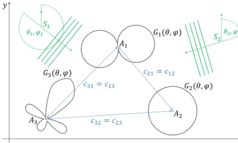
Figure 1.Schematic of an arbitrary array, antenna elements with arbitrary directional patterns, two impinging plane waves and re-sulting fixed coupling coefficients.
2.1.5 Mutual coupling
Stutzman and Thiele (2012) sum up mutual coupling as ra-diation coupling between nearby antennas, interactions be-tween an antenna and nearby objects, and possible coupling inside a common feed network. Since there is no common feed network and for a first theoretical consideration we ne-glect the mechanical support structure, the mutual coupling is only represented by unwanted interchange of energy be-tween each element in the array.
Even a perfectly matched dipole antenna in free space re-radiates or scatters as much power as it receives (Pozar, 2004). How much power is scattered or re-radiated depends on the antenna type, its relation to the ground plane and its impedance matching. In most applications antennas scatter more energy than they receive (Steyskal, 2010). The amount of coupled power depends on the radiation characteristic of each element, relative separation between each element and relative orientation of each element in an array (Balanis, 2005).
Figure 1 shows a representation of a receiving arbitrary planar array and elements with various antenna patterns. Now imagine impinging waves that induce currents. Power is absorbed by the antenna elements, some amount of power is re-radiated by each element and will be scattered to the neighbor elements. The scattered power will be received in each neighboring element additional to the impinging waves. This process theoretical repeats infinitely, but will decay very fast. This process will result in a sinusoidal excitation with an arbitrary amplitude|cij|and phase arg(cij)in antenna
el-ementicaused by elementj.
For most antenna types, due to the total spacing between antenna elements of at least dij ≥0.5λ, one can model the
interchange of energy as electromagnetic wave propagation. With a maximum phase deviation ofπ/8 the far-field starts at a distance ofR > λ/2 in case of anλ/2-dipole antenna el-ement (Balanis, 2005). Furthermore, this assumption factors
the directivity, polarization and orientation of the antenna el-ements to each other. With a fixed geometry of the array in-cluding the antenna’s orientations, the amplitude|cij|and the
phase shift arg(cij)of superimposed waves should be
con-stant. Examining Fig. 1, the forward and backward energy transfer from elementito elementjshould be equal.
Thus the discussed mutual coupling parameters can be de-fined as additional symmetric matrixC∈CM×M with
[C]ij = (
1 i=j cij i6=j
(6)
cij =cj i (7)
2.1.6 Support structure
Regarding the support structure, the dominant effects are coupling, refraction and diffraction. Complementary to the discussion in Sect. 2.1.5, the coupling between antenna el-ements and the mechanical support structure could proba-bly included in the mutual coupling matrixC. But refraction and diffraction, caused by mechanical support structure in the “field of view of the antenna elements” (FOVA), will not be solvable without a numerical analysis or extensive modi-fications in the data model.
Thus the best solution is to avoid mechanical support structure in the FOVA. In a linear patch antenna array this is satisfied a priori. In any array geometry like circular arrays or if dipole antennas with omnidirectional patterns are used with central feeding, this rule is violated.
The use of axially symmetric antennas like a bazooka dipole antenna could be a solution. Such antennas can be fed from the bottom and do not need support structure in the (FOVA). For example, Ott and Eibert (2010) presented a very broadband dipole antenna which is fed on the bottom side and which is axially symmetric.
2.1.7 Used data model
Based on the foregoing thoughts, the data model presented by Friedlander and Weiss (1991) is adequate, if the elements have a true omnidrectional pattern. Consider a receiving sit-uation as depicted in Fig. 1, withP narrow-band signals im-pinging on an array withMelements. This leads to the data model
X=C·0·A·S+N (8)
respectively
X=C·0·eA·S+N (9)
in S∈CP×K withK samples taken by the analog-digital-converter in the receiver. For the array’s response to each signal a steering-vector matrixA,eA∈CM×P is defined as
A= [a(θ1),a(θ2). . .a(θP)] (10) e
A=[ea(θ1),ea(θ2). . .ea(θP)] (11)
The sampled received signal matrix X∈CM×K is super-imposed by additive white gaussian noise (AWGN) inN∈
CM×K. Many calibration algorithms only consider one error
matrix for both mutual coupling and gain and phase errors of the antenna elements. This assumption coincides with all our thoughts in Sect. 2.1. An alternative representation of Eq. (8) is
X=4·A·S+N (12)
4= [ξ]ij=C·0 (13)
and will be used to compare different calibration algorithms in Sect. 3.
2.1.8 DOA estimation
There are a lot of modifications of well known algorithms, which can be used for DOA estimation. In this paper we use the standard MUSIC algorithm (Schmidt, 1986), adapted to the data models in Eqs. (8) and (9). The DOA spectrum is calculated by
PMU(θ )=
EHN·C·0·a(θ )
−2
2 (14)
PMU(θ )=
EHN·C·0·ea(θ )
−2
2 (15)
where (·)H means the Hermitian transponse and EN∈
CM×(M−P ) is matrix whose columns are theM−P noise
eigenvectors.
Nearly every estimation algorithm can be adapted to this data model. To demonstrate this, the older estimation algo-rithm CAPON (Capon, 1969) can be extended to
PCP(θ )=
aH(θ )·0H·CH·RXX−1·C·0·a(θ ) −1
(16) But this is only for your interest of DOA estimation and shall not be treated more in detail. Just keep in mind that well known DOA estimation algorithms can be adapted to the used data model for array calibration.
2.2 Appraisals of error quantities
As mentioned before, we want to estimate the error quantities like mutual coupling and gain and phase errors of antenna elements, for example of a linear array with patch antenna elements and a circular array with dipole elements.
Some calibration algorithms consider possible antenna el-ement position errors, but we do not take these into account.
Table 1.Calculated coupling quantities for dipole antennas in an arbitrary array and patch antenna elements in a linear array with different distances relative to wavelength.
d12 0.5λ 0.6λ 0.7λ 0.8λ
|cPatch| 0.08 0.06 0.05 0.05 |cDipole| 0.26 0.22 0.19 0.16
A given position error of an element of 0.5 mm, which is for a production facility a great tolerance, with
18=2πδdmax
λ (17)
would lead to a maximum phase error of 1.8◦ at 3 GHz. Therefore, the errors due to positioning error are very small compared to other error sources and will be omitted in the following treatment.
For the gain error of a sensor we assumed up to 5 %, which leads to a gain correction factor ofαm= [0.95,1.05]
in Eq. (5). Maximum phase errors of υm= ±20◦ are
ex-pected.
In Sect. 2.1.5 we modeled the interchange of energy be-tween antenna elements as electromagnetic wave propaga-tion, due to the far-field region for distancesR > λ/2 in case ofλ/2-dipole antenna elements. The link budget of a trans-mitting and a receiving antenna with far-field conditions can be calculated by the Friis transmission equation. Therefore, we estimate the coupling coefficients by
|cij| ≈ s
PTX−j
PRX−i =
s
Gi(θj)·Gj(θi)·λ2
(4π·dij)2
(18)
arg(cij)≈ −
2π·dij
λ (19)
whereGi(θj)is the antenna gain of elementiin direction to
antenna elementj,Gj(θi)is the gain of elementj in
direc-tion to antennai, anddij is the total distance between those
two elements. These results are not precise values, but for an estimation withdij ≥λ2 it is sufficient.
Typical antenna gain for λ2-dipole antenna is 2.15 dB. A built patch antenna, as shown in Sect. 4, has a simulated an-tenna gain of−3.24 dB atθ=90◦andθ= −90◦. Coupling quantities calculated by Eq. (18) for a linear patch antenna array and a circular dipole array are shown in Table 1. A sim-ulation of these arrays with CST confirms the estimation re-sults and covers with rere-sults presented by Gupta et al. (2003).
3 Evaluation of some calibration algorithms 3.1 Overview
All of them consider mutual coupling as well as sensor gain and phase errors. Algorithms which consider possible po-sition errors shown in Weiss and Friedlander (1988), Hung (2000) and Ng and See (1996) are not analyzed.
Pierre and Kaveh (1991) proposed a method which con-ducts a direct quadratic minimization for estimating4. Mea-surements were done on an acoustic ultrasonic array test-bed (Pierre and Kaveh, 1995). Subsequent we will call this method direct-quadratic-minimization (DQM).
See (1994) used the DQM as starting point and extended the method by an complex scaling vector3for optimized re-sults in4. This method will be denominated extended-direct-quadratic-minimization (EDQM).
A further optimization of the DQM and the EDQM meth-ods was proposed by Jaffer (2001). He assumed that the cou-pling coefficients are|cij| =0 for farther antenna elements.
The algorithm is computationally more efficient than DQM and EDQM, but we do not evaluate this algorithm because we do not want to neglect the coupling influences caused by dipole elements in a circular array.
Friedlander and Weiss (1991) presented a well known and often cited auto-calibration method, which is able to per-form the calibration without knowledge of the calibration sources’ positions. It has to be assured that at least two target sources are sending at the same time while the calibration is performed. From Hung (1994) we know that the method can be inaccurate and Pierre and Kaveh (1991) showed that the method will not work for linear arrays. Nevertheless, we evaluate this method due to its high popularity. In the fol-lowing, the method will be called auto-calibration-method (ACM).
3.2 Evaluation
In Sect. 2.2 we estimated mutual coupling coefficients and possible gain and phase errors in the antenna elements. With those estimated quantities inserted in Eq. (13), we get max(|ξij|)=0.274. That means that the mentioned
calibra-tion algorithms must be able to estimate error quantities up to max(|ξij|)=0.274 for elements withdij =λ2.
The evaluation procedure was done as follows. The sym-metric coupling matrix Ccan be modeled to be a Toeplitz matrix in case of a linear array and a cyclic matrix in case of a circular array (Friedlander and Weiss, 1991). Based on these thoughts, we generated Cwith|c21| in the range
be-tween 0.01 and 0.4.0was calculated by Eq. (5) and with
αm=1.0+0.05·σα (20)
υm=
20◦·π
180◦ συ (21)
whereσα andσυare a Gaussian distribution with zero mean.
With a step size for|c21| of 0.01, we generated simulation
data with Eq. (8). At each step 20 simulations were run and the DQM, EDQM and the ACM were used to solve 4 re-spectively Cand0. A deviation between simulated 4and
0 0.1 0.2 0.3 0.4 0.5
j921j 0
0.5 1 1.5 2 2.5 3
"
%
Simulated "% as function of |9
21|
"%DQM "%EDQM "%AKM
Figure 2.Mean of14of simulated DQM, EDQM and ACM algo-rithm with 20 cycles and step size 0.01.
0 0.1 0.2 0.3 0.4 0.5
j921j 0
2 4 6 8 10
"
3R
M
S
[
/]
Simulated "3
RMS as function of |921|
"#RMSDQM "#RMSEDQM "#RMSACM
Figure 3.Mean of1θRMSof simulated DQM, EDQM and ACM algorithm with 20 cycles and step size 0.01.
estimated4ˆ by the algorithms was calculated by
14= k ˆ4−4kF (22)
wherek · kFis the Frobenius norm. As an additional bench-mark, the MUSIC algorithm was used to estimate the DOA on 180 simulated target directions with the estimated4ˆ in Eq. (14) in each simulation. Finally, the root mean squared DOA error was calculated by
1θRMS= q
(θˆ−θ )2 (23)
Figure 2 shows the mean and standard deviation of14 and Fig. 3 the same with1θRMS of 20 simulation runs on
-100 -50 0 50 100 Direction-of-arrival 3 [°]
0 10 20 30 40 50 60 70 80 90
MUSIC spectra [dB]
EDQM calibration on linear patch antenna array
No calibration
Omnidirectional patterns Directional patterns
Figure 4.MUSIC spectra of a linear array with patch antenna el-ements with uncalibrated manifold, with calibrated manifold with omnidirectional patterns, and calibrated manifold with directional antenna patterns.
method provides the worst results and is very fragile com-pared to its enhancement the EDQM method. The EDQM method is very stable in the simulated error range and pro-vides the best1θRMSvalues over the full simulation range.
The DQM method’s14is linearly dependent from|ξ21|
and does not provide reliable calibration values for |ξ21|>
0.2. Friedlander’s ACM delivers solid DOA estimation val-ues in the simulated range. Nevertheless the14quality has an optimum point around |ξ21| =0.23. This optimum
de-pends on the choosen linear contraints and can be set up. Fi-nally, the EDQM method provides stable and reliable results and delivers accurate DOA estimations. Our focus is clearly set on the EDQM method.
3.3 Simulations with directional antenna patterns
For the sake of completeness, the EDQM calibration algo-rithm were tested again with directional antenna patterns. Therefore, the antenna gain was simulated for printed PCB dipole antennas in a circular array and patch antennas in a linear array in CST. The simulated antenna patterns were im-pressed on the ideal manifolds with Eq. (3). Several sim-ulations were performed with data generated according to Eq. (9).
Figure 4 gives information about estimated MUSIC spec-tra without calibration, the specspec-tra with calibration process using Eq. (1), and the spectra with calibration process using Eq. (3) on a linear array with patch antennas. Without using a calibration algorithm, the peaks are blurred. A calibration process using the ideal manifold or the weighted manifold leads to higher and sharper peaks. The same result is pro-vided in a second simulation with a circular array with PCB dipole antenna elements, shown in Fig. 5.
0 50 100 150 200 250 300 350
Direction-of-arrival3[/]
0 10 20 30 40 50 60 70
M
U
S
IC
sp
ec
tr
a
[d
B
]
EDQM calibration on circular PCB dipole antenna array
No calibration
Omnidirectional patterns Directional patterns
^
3p ^
3p
Figure 5.MUSIC spectra of circular array with simulated PCB dipole elements with uncalibrated manifold, with calibrated man-ifold with omnidirectional patterns, and calibrated manman-ifold with directional antenna patterns.
Figure 6.Built linear patch antenna array with 4 elements.
Another aspect we can see in Fig. 4 is that the peaks for the calibration with omnidirectional patterns and the calibration with directional patterns have the same height. This can be explained by the same orientation of each ideal patch antenna which leads to equal directivity as function of the DOA. But for the circular array simulation, we oriented the elliptical pattern of the PCB dipole elements starlike. Thus, the differ-ent oridiffer-entated patterns lead to differdiffer-ent amplitude scaling fac-tors in dependency of the DOA. Therefore, the peaks of di-rectional pattern calibration are sharper and higher in Fig. 5.
4 Measurements
off-the-Figure 7.Built circular bazooka dipole array with 7 elements.
Figure 8.Picture of the measurement setup in an open wide and flat meadow area for far-field measurements.
shelf antennas. We discussed in Sect. 2.1.6 that it is best to avoid mechanical structures in the FOVA. Thus, we built a linear antenna array with four quadratic patch antenna el-ements shown in Fig. 6, and a circular array with seven bazooka dipole elements depicted in Fig. 7.
The total antenna spacing in the linear array is 0.5λand in the circular array 0.65λ. For the down conversion we used a coherent eight-channel receiver with integrated calibration capability. Our operating frequency isf0=867 MHz with a
wavelength ofλ0=345.78 mm.
Both antenna arrays were placed on an open wide and flat meadow area for far-field measurements, see Fig. 8. With a transmitting oscillator running at 867 MHz at a fixed posi-tion and rotating the complete array, the complete manifold of both antenna arrays were measured. Then we chose 9 cal-culated steering vectorsameas(θi)of the measured manifold
of the 4-element linear array and applied the EDQM method.
Figure 9.Shape of 4-element linear patch array, element 3, the ideal manifold, the measured manifold and the calculated manifold by calibration method EDQM.
For the 7-element circular array we chose 11 measured steer-ing vectors. The measured steersteer-ing vectorsameas(θi)were
calculated by an eigenvalue decomposition of the signal co-variance matrix by
RXX=
1 K
X
XXH= M X
i=1
λieˆieˆHi →ameas∝ ˆe1 (24)
in whicheˆiis theith eigenvector after sorting them, by their
eigenvalues in descending order.
Figure 10.Shape of 7-element circular dipole array, element 4, the ideal manifold, the measured manifold and the calculated manifold by calibration method EDQM.
and follows the measured phase. Same result can be achieved with the circular array in Fig. 10.
Nevertheless, the summary is, that calibration algorithms do not deliver such accurate phase and amplitude calibra-tion values, which are needed for the use of high resolucalibra-tion DOA algorithms like MUSIC. It is to suspect that some error source that is not yet modeled in Eq. (9) is present.
5 A new effect in modeling errors
A regular assumption made by all authors is the constant am-plitude during the wave propagation over the antenna array. The assumption is based on the idea that the target sources are much farther away than the greatest distance between the antenna elements in the array. But this assumption im-plies that each antenna element has “its own plane wave front” which impinges on the antenna element and receives the same amount of energy.
Figure 11.Monitored electric field strength around a dipole antenna with an impinging plane wave front, direct 2-D-field perspective, propagation direction from the left to the right.
Figure 12.Monitored electric field strength around a λ2-dipole an-tenna with an impinging plane wave front, curve along the propaga-tion direcpropaga-tion near the dipole antenna,f0=867 MHz.
In an arbitrary array with different directionsθ, there is always an element which is “closer on the wave front” and some elements which are “farther away” due to their posi-tion behind the first element. If the wave front impinges on the effective area of the first antenna element, the antenna absorbs energy from the propagating electromagnetic field. That leads to the question if it is possible that there can be as much energy for the second antenna element as for the first one. This should not be possible because the first antenna absorbs energy out of the field, which is now not available anymore for antenna elements behind the first one.
su-perposition of the impinging field and the re-radiated field by the antenna due to the induced currents.
In Fig. 12, in the area between 0 and 1000 mm one can clearly observe the constructive and destructive interference of impinging and re-radiated electromagnetic waves. After passing the dipole antenna, the enfeebled propagating plane wave and the re-radiated wave by the antenna are in phase. The interference should be constructive in the whole area be-tween 1000 and 2000 mm, but the simulation shows that the electric field strength in the right half-space is even smaller than 1 V m−1. This result confirms the suspicion that the propagating electromagnet field contains not as much energy after passing the first antenna element as before.
The antenna element causes a shadowing effect of the im-pinging wave front for the local area behind the antenna in propagation direction, superimposed by the re-radiation of the induced currents. It is quite intuitive that the amount of energy stored in the electromagnetic field can not be the same behind the antenna, if power is delivered on the antenna ter-minal. But this means that the assumption is not correct, that every antenna element receives electromagnetic energy with same amplitude. All available energy in the local area of the antenna array must be splitted up for every antenna element of the array.
The described behavior does not fit on the regular used data model in Eqs. (8) and (9). This discrepancy would explain why many calibration algorithms exhibit problems when dealing with real antenna arrays. The fact that in the linear array the calibration algorithm were more successful than in the circular array solidifies this theory. Due to the side-by-side placement of the patch antenna elements, the shadowing effect is not as distinct as in the circular array. This can be clearly seen in Figs. 9 and 10.
If it is possible to determine a mapping of this local shad-owing effect, which is a function of DOA(θ ), antenna gain G(θ ), and initially the array geometry(xm, ym), similar toC
anda(θ ), which we define as
ψm(θ ) (25)
9(θ )= [ψ1(θ ), ψ2(θ ). . .ψM(θ )]T (26)
where 9(θ )∈RM×1 is a scaling function for the received signal amplitude on each channel. The data model should be extended to
a9(θ )=9(θ )◦f(θ )◦a(θ ) (27)
A9= [a9(θ1),a9(θ2). . .a9(θP)] (28)
X=C·0·A9·S+N (29)
to consider the split of electromagnetic energy, which is available in the local area, in unequal portions for each ar-ray element.
6 Conclusions
In this paper we discussed the regularly used data model for direction-of-arrival estimation extensively. A deep insight into the known error sources was given and further require-ments on the array design were presented. Further we figured out that the model is conclusive to its mutual coupling matrix and the gain and phase error matrix.
Well known calibration algorithms were analyzed for its robustness to estimated error quantities. A linear antenna patch array and a circular dipole antenna array were built which avoid refraction and diffraction caused by the sup-port structure. Measurement results were presented, which showed that the calibration algorithms were not able to cor-rect the induced errors.
A new effect in modeling errors due to shadowing caused by nearby antennas was presented and discussed. Electro-magnetic field simulations have been made to substantiate the modeling error. A possible adaption of the data model has been proposed. Future work is the investigation about the shadowing effect of antennas and derive an analytic function which calculates this effect.
Acknowledgements. The project is supported by funds of the
Federal Ministry of Food, Agriculture and Consumer Protection (BMELV) based on a decision of the Parliament of the Federal Republic of Germany via the Federal Office for Agriculture and Food (BLE) under the innovation support programme.
This work was supported by the German Research Foundation (DFG) and the Technische Universität München within the funding programme Open Access Publishing.
Edited by: R. Schuhmann
Reviewed by: two anonymous referees
References
Balanis, C. A.: Antenna theory: analysis and design, 3rd Edn., John Wiley & Sons, Hoboken, USA, 2005.
Capon, J.: High-resolution frequency-wavenumber spectrum analy-sis, Proc. IEEE, 57, 1408–1418, doi:10.1109/PROC.1969.7278, 1969.
Eberhardt, M., Ascher, A., Lehner, M., and Biebl, E.: Array Man-ifold Manipulation for Short Distance DOA Estimation with a Handheld Device, Smart SysTech 2015, European Conference on Smart Objects, Systems and Technologies, 1–7, 2015a. Eberhardt, M., Lehner, M., Ascher, A., Allwang, M., and Biebl, E.
Grabau, R.: Funkpeiltechnik: Grundlagen-Verfahren und An-wendungen, peilen-orten-navigieren-leiten-verfolgen, Franckh, 1989.
Gupta, I., Baxter, J., Ellingson, S., Park, H.-G., Oh, H. S., and Kyeong, M. G.: An experimental study of antenna array calibration, IEEE T. Antenn. Propag., 51, 664–667, doi:10.1109/TAP.2003.809870, 2003.
Hung, E.: A critical study of a self-calibrating direction-finding method for arrays, IEEE T. Signal Proces., 42, 471–474, doi:10.1109/78.275633, 1994.
Hung, E.: Matrix-construction calibration method for an-tenna arrays, IEEE T. Aero Elec. Sys., 36, 819–828, doi:10.1109/7.869501, 2000.
Jaffer, A.: Constrained mutual coupling estimation for array calibration, Conference Record of the 35th Asilomar Con-ference Signals, Systems and Computers, 2, 1273–1277, doi:10.1109/ACSSC.2001.987695, 2001.
Loibl, C. and Biebl, E.: Localization of passive UHF RFID tagged goods with the Monopulse principle for a logistic application, Proceedings of 2012 European Conference on Smart Objects, Systems and Technologies (SmartSysTech), 1–5, 2012. Morhart, C., Biebl, E., Schwarz, D., and Rasshofer, R.: Cooperative
Multi-User Detection and Localization for Pedestrian Protection, 2009 German Microwave Conference, Munich, Germany, 16–18 March 2009, 1–5, doi:10.1109/GEMIC.2009.4815863, 2009. Ng, B. C. and See, C. M. S.: Sensor-array calibration using
a maximum-likelihood approach, Antennas and Propagation, IEEE T. Antenn. Propag., 44, 827–835, doi:10.1109/8.509886, 1996.
Ott, A. and Eibert, T.: A 433 MHz-22 GHz reconfigurable dielectric loaded biconical antenna, 2010 Proceedings of the Fourth Euro-pean Conference on Antennas and Propagation (EuCAP), 1–5, 2010.
Pierre, J. and Kaveh, M.: Experimental performance of calibration and direction-finding algorithms, 1991 International Conference on Acoustics, Speech, and Signal Processing, ICASSP-91, 2, 1365–1368, doi:10.1109/ICASSP.1991.150676, 1991.
Pierre, J. and Kaveh, M.: Experimental Evaluation of High-Resolution Direction-Finding Algorithms Using a Calibrated Sensor Array Testbed, Digit. Signal Process., 5, 243–254, doi:10.1006/dspr.1995.1024, 1995.
Pozar, D.: Scattered and absorbed powers in receiving antennas, IEEE Antenn. Propag. M., 46, 144–145, doi:10.1109/MAP.2004.1296172, 2004.
Schmidt, R.: Multiple emitter location and signal parame-ter estimation, IEEE T. Antenn. Propag., 34, 276–280, doi:10.1109/TAP.1986.1143830, 1986.
Schmidt, R. and Franks, R.: Multiple source DF signal processing: An experimental system, IEEE T. Antenn. Propag., 34, 281–290, doi:10.1109/TAP.1986.1143815, 1986.
See, C.: Sensor array calibration in the presence of mutual coupling and unknown sensor gains and phases, Electro. Lett., 30, 373– 374, doi:10.1049/el:19940288, 1994.
Steyskal, H.: On the Power Absorbed and Scattered by an Antenna, IEEE Antenn. Propag. M., 52, 41–45, doi:10.1109/MAP.2010.5723219, 2010.
Stutzman, W. L. and Thiele, G. A.: Antenna theory and design, John Wiley & Sons, Hoboken, USA, 2012.
Tuncer, E. and Friedlander, B.: Classical and Modern Direction-of-Arrival Estimation, Academic Press, Burlington, USA, 2009. Weiss, A. and Friedlander, B.: Array shape calibration