R E S E A R C H
Open Access
A framework for the extended evaluation
of ABAC policies
Charles Morisset
1, Tim A. C. Willemse
2and Nicola Zannone
2*Abstract
A main challenge of attribute-based access control (ABAC) is the handling of missing information. Several studies have shown that the way standard ABAC mechanisms, e.g. based on XACML, handle missing information is flawed, making ABAC policies vulnerable to attribute-hiding attacks. Recent work has addressed the problem of missing information in ABAC by introducing the notion of extended evaluation, where the evaluation of a query considers all queries that can be obtained by extending the initial query. This method counters attribute-hiding attacks, but a naïve implementation is intractable, as it requires an evaluation of the whole query space. In this paper, we present a framework for the extended evaluation of ABAC policies. The framework relies on Binary Decision Diagram (BDDs) data structures for the efficient computation of the extended evaluation of ABAC policies. We also introduce the notion of query constraints and attribute value power to avoid evaluating queries that do not represent a valid state of the system and to identify which attribute values should be considered in the computation of the extended evaluation, respectively. We illustrate our framework using three real-world policies, which would be intractable with the original method but which are analyzed in seconds using our framework.
Keywords: Attribute-based access control, Policy evaluation, Missing attributes, Attribute power, Attribute-hiding attacks
Introduction
Attribute-Based Access Control (ABAC) is emerging as the de facto paradigm for the specification and enforce-ment of access control policies. In ABAC, policies and access requests are defined in terms of attribute name-value pairs. This provides an expressive, flexible and scalable paradigm that is able to capture and manage authorizations in complex environments.
Although ABAC provides a powerful paradigm for access control, ABAC systems require that all the infor-mation necessary for policy evaluation is available to the policy decision point, which might be difficult to achieve in modern systems. Recent years have seen the emergence of authorization mechanisms that go beyond the view of a centralized monitor with full knowledge of the system. Authorization mechanisms increasingly rely on external services to gather the information necessary for access decision making (e.g., Amazon Web Services rely on
*Correspondence:[email protected]
2
Eindhoven University of Technology, P.O. Box 513, 5600 MB, Eindhoven, Netherlands
Full list of author information is available at the end of the article
third-party identity providers and federated identity systems, the OAuth 2.0 protocol enables delegation of authorization). The use of external information sources for attribute retrieval makes it difficult to guarantee and, in some cases, even to check that all necessary informa-tion has been provided. Moreover, in some domains like IoT, it might be difficult and costly to gather (accurate) information needed for policy evaluation. Missing infor-mation can significantly influence query evaluation and pose significant risks to a large range of modern systems.
To this end, existing ABAC models are often equipped with mechanisms to handle missing attributes during pol-icy evaluation.
However, these mechanisms have some intrinsic drawbacks (Crampton and Huth2010; Tschantz and Krishnamurthi 2006). For instance, eXtensible Access Control Markup Language (XACML) (OASIS2013), the de facto standard for the specification and evaluation of ABAC policies, pro-vides a mechanism to deal with missing attributes. How-ever, Crampton et al. (2015) showed that the evaluation of a XACML query can yield a decision that does not necessarily provide an intuitive interpretation on whether
access should be granted or not due to the fact that some information needed for the evaluation might be missing. These drawbacks make the evaluation of ABAC policies vulnerable to attribute hiding attacks where users can obtain a more favorable decision by hiding some of their attributes (Crampton and Morisset2012).
To make the evaluation of ABAC policies robust against attribute hiding attacks, previous work (Crampton et al. 2015) has proposed a novel approach that allows for an extended evaluation of ABAC policies.
In a nutshell, the authors suggest that the evaluation of a given query is calculated using the evaluation of all queries that can be constructed from the initial query. This way, the extended evaluation unveils the risks when informa-tion could be, inteninforma-tionally or not, hidden to the policy decision point. However, this approach requires exploring the state space for all possible queries, which is exponen-tial in the number of attribute values, and therefore not particularly efficient.
In this work, we present a formal framework for the extended evaluation of ABAC policies that addresses this drawback, extending our previous work (Morisset et al. 2018). Our framework includes several evaluation meth-ods, as well as the notions of query constraint, which is used to exclude those queries that are not possible within the system from the query space. Our framework relies on binary decision diagram (BDD)-based data structures for the encoding ABAC policies. As shown in previous work (Bahrak et al.2010; Fisler et al.2005; Hu et al.2013), these data structures provide a compact encoding for storing the decisions yielded by an ABAC policy for every query and for efficient policy evaluation. Moreover, the frame-work is equipped with an efficient method to compute the extended evaluation directly on the BDD structure. To further optimize the computation of the extended evalua-tion, we also introduce the notion ofattribute value power, which provides insights into the impact of attributes on decision making. This can help determine which attribute should be considered in the computation of the extended evaluation by excluding attribute values when they have no power (i.e., they have no impact on decision making). To the best of our knowledge, this is the first work that investigates the impact of attributes on the evaluation of ABAC policies.
We demonstrate our approach on three complex case studies, where a naïve approach would deal with a query space comprising several millions of states, whereas our approach compiles in a few seconds a compact decision diagram. Compared to Morisset et al. (2018), we also ana-lyze the time required for policy evaluation using BDD data structures and we show that our framework out-performs SAT-based policy frameworks. Moreover, we present a quantitative analysis of the attribute value power for the three case studies.
The remainder of this paper is organized as follows. The next section presents preliminaries on ABAC and the no tion of extended evaluation. “Problem statement” section introduces a motivating example and provides a for-mulation of the problem. “Query constraints” section presents the notion of query constraint. “Attribute power” section presents the notion of attribute value power. “Efficient extended evaluation computation” section pres-ents a novel algorithm to compute the extended query evaluation. “Case studies” section provides a valida-tion of our approach on three real-world policies. Finally, “Related work” section discusses related work and “Conclusion” section concludes the paper. We provide the proofs of the theorems in appendix.
Preliminaries
This section presents a general view of how Attribute-Based Access Control (ABAC) policies and queries are evaluated using PTaCL (Crampton and Morisset 2012), which provides an abstraction of the XACML standard (OASIS 2013). We first present the syntax of PTaCL, which encompasses two different languages: one for tar-gets, which is used to decide the applicability of a policy to a query, and another for policies, which is used to spec-ify how policies are combined together. We then present two evaluation functions proposed for PTaCL: the stan-dard evaluation function, introduced in Crampton and Morisset (2012) and the extended evaluation function, introduced in Crampton et al. (2015).
ABAC syntax
In ABAC, queries and policies are defined in terms of attribute name-value pairs (instead of the traditional triple subject, object, access mode). More precisely, let A = {a1,. . .,an} be a finite set of attributes, and given an attribute a ∈ A, let Va be the domain of a. The set of queries QA is then defined as ℘ (⋃ni=1ai× Vai), and
a query q = {(a1,v1),. . .,(ak,vk)} is a set of attribute name-value pairs (ai,vi)such thatai ∈ Aandvi ∈ Vai.
A query encompasses both a specific request for access, and a current view of the world describing the different entities concerned by that request.
The PTaCL language istree-based, i.e. policies are recur-sively constructed from atomic policies using operators. This vision follows the traditional “separation of concerns” principle: each policy might regulate accesses to a specific sub-domain of an organization, or regulate accesses done by a specific category of users or in specific contexts. In order to identify which policies are applicable to which targets, PTaCL introduce a target languageTA, such that a targett∈ TAis defined as:
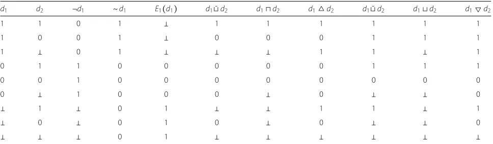
where(a,v)is an attribute name-value pair andopis ann -ary operator defined over the setD3= {1, 0,}, indicating that the target matches the query, that the target does not match the query, and that it is indeterminate whether the target matches the query or not (the semantical evaluation of targets is described below). Table1presents the oper-ators provided by PTaCL as well as operoper-ators commonly used in ABAC languages. It is worth noting that the set of operators{¬,E1, ˜⊔}is canonically complete (Cramp-ton and Williams2016), i.e. any 3-valued operator can be constructed using these three operators.
PTaCL also defines a policy languagePA, where a policy p∈ PAis defined as:
p=1∣0∣ (t,p) ∣op(p1,. . .,pn)
where 1 and 0 represent the allow and deny decisions respectively, (t,p)is a target policy and op is an n-ary operator, also defined on the three-valued set {1, 0,}, whererepresents thenot-applicabledecision. Although this set is syntactically equivalent to the one used for tar-gets, the meaning of the values in the set depends on whether it is used as a target or as a policy. This should always be clear from the context in the remainder of this paper.
ABAC evaluation
Given the set of policiesPA, the set of queriesQA and a set of decisionsD, an evaluation function is a function ⋅∶ PA×QA→ Dsuch that, given a queryqand a policy p,p(q)represents the decision of evaluatingpagainstq. PTaCL has two main policy evaluation functions, which handle missing attributes in a different way. For the sake of uniformity, hereafter we might use different notations than those used in the original publications.
Standard evaluation
The standard evaluation consists in evaluating a target to when the attribute is completely missing from the query, to 0 if the attribute is present in the query, but without
the appropriate value, and to 1 otherwise. A policy then evaluates to a set of decisions withinD7= ℘({1, 0,})/∅ where 1 and 0 indicate that access should be granted or denied respectively, andthat the policy is not applicable to a given query.
Non-singleton decisions are returned when the query does not provide the information necessary to evalu-ate a target (i.e., the target evaluevalu-ates to ). Intuitively, non-singleton decisions correspond to theindeterminate decision in XACML (Morisset and Zannone2014).
More formally, the semantics of a targettis given by the function:
⋅T∶ TA×QA→ D3
(a,v)T(q) =⎧⎪⎪⎪⎨⎪⎪
⎪⎩
1 if(a,v) ∈q
if∀v′∈ Va∶ (a,v′) /∈q 0 otherwise
op(t1,. . .,tn)T(q) =op(t1T(q),. . .,tnT(q))
The standard semantics of a policy pis given by the function:
⋅P∶ PA×QA→ D7 1P(q) = {1}
0P(q) = {0}
(t,p)P(q) =⎧⎪⎪⎪⎨⎪⎪
⎪⎩
pP(q) iftT(q) =1
{} iftT(q) =0 {} ∪pP(q) otherwise op(p1,. . .,pn)P(q) =op↑(p1P(q),. . .,pnP(q))
where, given an operatorop∶ D3× D3→ D3and any non-empty setsX,Y ⊆ D3,op↑ ∶ D7× D7→ D7is defined as op↑(X,Y) = {op(x,y) ∣ x ∈X∧y ∈ Y}. Intuitively,op↑ corresponds to operatoropextended in a point-wise way to sets of decisions.
Table 1Operators on the setD3= {1, 0,}
d1 d2 ¬d1 ∼d1 E1(d1) d1⊔˜d2 d1⊓d2 d1△d2 d1⊔˜d2 d1⊔d2 d1▽d2
1 1 0 1 1 1 1 1 1 1
1 0 0 1 0 0 0 1 1 1
1 0 1 1 1 1
0 1 1 0 0 0 0 0 1 1 1
0 0 1 0 0 0 0 0 0 0 0
0 1 0 0 0 0 0
1 0 1 1 1 1
0 0 1 0 0 0
Extended evaluation
The extended evaluation relies on a non-deterministic attribute retrieval (Crampton et al. 2015)1. The funda-mental intuition is to model the fact that a query might represent a partial view of the world, whereby some attribute values are missing.
The extended evaluation of an ABAC policy is com-puted using two functions: thesimplifiedevaluation func-tion and theextendedevaluation function. The simplified evaluation function ⋅ ignores missing attributes,2 and therefore always returns a single decision. Formally:
⋅B∶ PA×QA→ D3 1B(q) =1
0B(q) =0
(t,p)B(q) = {pB(q) ifotherwisetT(q) =1
op(p1,. . .,pn)B(q) =op(p1B(q),. . .,pnB(q))
The extended evaluation function evaluates a query to all possible decisions that can be obtained by adding pos-sibly missing attributes. Hereafter, we represent a query space as a directed acyclic graph (save for self-loops) (QA,→), whereQAis a set of queries, and→⊆QA×QA is a relation such that, given two queriesq,q′∈QA,q→q′ if and only ifq′=q∪ {(a,v)}for some attributea∈ Aand some valuev∈ A.
Note that some extensions of a queryqmay not be pos-sible. For instance, for a given Boolean attribute, it might not make sense to have in the same query bothtrueand falsefor that attribute. Hence, Crampton et al. introduce in Crampton et al. (2015) the notion of negative attribute value to explicitly indicate that an attribute cannot have a certain value in a given context and the notion of well-formed predicatewf∶QA→Bover queries to ensure that a query does not contain both an attribute value and its negation.
Based on these notions, the extended evaluation func-tion⋅Eis defined as follows:
⋅E∶ PA×QA→ D8= ℘({1, 0,}) pE(q) = {pB(q′) ∣q→∗q′∧wf(q′)}
where →∗ denotes the reflexive-transitive closure of→. With the restrictions imposed on →, the relation →∗ reduces to the subset relation on queries. It is worth observing that ⋅E returns the empty set for any query that does not satisfy wf. In “Query constraints” section we will refine predicate wf by introducing the notion of query constraint to capture more complex domain requirements.
Problem statement
We illustrate the drawbacks of the standard and extended evaluation functions through a sample policy. Consider a system wherein access is based on the nationality of users. In particular, the system allows Belgians to access system resources, whereas the Dutch are not. This policy can be represented as follows:
p= ((nat,BE), 1)((nat,NL), 0)
Standard evaluation function ⋅P: Crampton et al. (2015) have shown that the standard evaluation, which is the one used by XACML, can yield a decision that does not necessarily provide an intuitive interpretation on whether access should be granted or not due to the fact that some information needed for the evaluation might be missing. In other words, given a policy, it is possi-ble for a query to evaluate to a set of decisions Dsuch that there exists a decision d ∈ Dfor which the query extended with additional attribute values would not eval-uate tod, while there could be some decisiond′ ∉Dfor which the query extended with some additional attribute values would evaluate tod′. We exemplify these issues in the following example.
Consider a user submitting the queryq = {(nat,BE)}, stating that the user is Belgian. This query evaluates pP({(nat,BE)}) = {1}, i.e. the access is granted. How-ever, it is possible for a user to have multiple nation-alities, and in some cases, it might be possible for a user to hide some nationalities3. In our case, the user might be hiding that she also has a Dutch nationality, in which case the access should have been denied since pP({(nat,BE),(nat,NL)}) = {0}.
Extended evaluation function ⋅E: To overcome the drawbacks of function⋅P, given a policypand a query
q, a policy enforcement point (i.e., the point in the system in charge of enabling an access query or not) can evaluate pE(q)in addition topB(q), to determine whether any missing attribute could change the evaluation. In partic-ular, we obtainpE({(nat,BE)}) = {1, 0}indicating that there exists a query (i.e., a view of the world) reachable fromqthat should be denied.
Computing pE(q), however, requires evaluating all queries that can be constructed from the initial queryq. This leads to two main problems:
– A naïve implementation of⋅Erequires exploring a
very large query space, making policy evaluation inefficient.
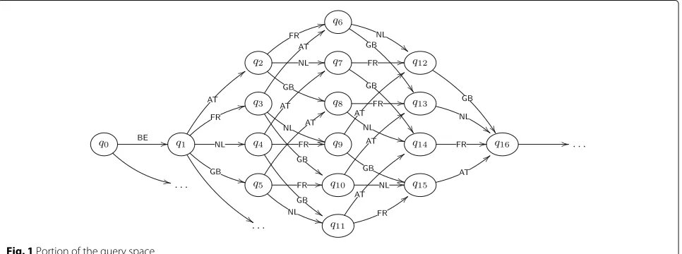
To visually represent these problems, consider (the por-tion of ) the query space in Fig.1, which is explored in the evaluation of queryq. In the figure, nodes represent queries (withq0the empty query) and edges are annotated with a label indicating how a query has been extended, i.e. qiNL→qjdenotesqj=qi∪ {(nat,NL)}.
Concerning the first problem, we have to account that there are 206 sovereign states recognized by the United Nations4, and users can have more than one nation-ality. Therefore, computing pE(q) requires evaluating 2205 queries (i.e., the queries that can be constructed from the initial query {(nat,BE)}), which is clearly infeasible.
More importantly, ignoring domain constraints can result in decisions that cannot be reached in practice, thus providing misleading information for decision making. We illustrate this using two examples.
Although there is no limit on the number of nationali-ties individuals can hold according to international laws, it is reasonable to assume that this number is limited. For the sake of exemplification, let us assume that individuals cannot hold more than three nationalities.
According to this domain constraint, no queries formed by four or more attribute name-value pairs are reach-able from the initial state (i.e., queries q12 to q16 in Fig. 1) as they are not plausible views of the world. If those queries are evaluated, the access control system can return decision that cannot be reached in practice. For instance, considerq10 = {(nat,BE),(nat,GB),(nat,FR)}. The (simplified) evaluation ofq10against policypreturns apermitdecision, i.e.pB(q10) = {1}. However, ignor-ing domain constraints, we havepE(q10) = {1, 0}. In fact, the extended evaluation of q10 requires evaluating
q15 =q10∪ {(nat,NL)}, which however is not a plausible view of the system according to the domain requirement.
As another example, one can consider that several countries have constraints on double nationality. Suppose,
for instance, that Austria does not allow dual national-ity with the Netherlands5. In this case, we should exclude from the state space any query containing both attribute name-value pairs(nat,NL)and(nat,AT)(i.e., queriesq7,
q12, q14 andq16 in Fig.1). Accordingly, given the query
{(nat,AT)}, we expect this request to be never denied, even if some attribute is missing.
In contrast, if domain constraints are neglected, we obtainpE({(nat,AT)}) = {1, 0,}.
Contribution In the remainder of the paper, we will exploit these observations to establish the foundations for the design of practical policy frameworks supporting the extended evaluation of attribute-based access control policies. In particular:
– We introduce the notion ofquery constraint to identify which views of the world are plausible based on domain specific requirements and assumptions, thus constructing a realistic query space (“Query constraints” section).
– We introduce the notion ofattribute value power to determine how much an attribute value is capable of triggering a specific decision (“Attribute power” section).
– We investigate practical approaches for the computation of the extended evaluation function
⋅E(“Efficient extended evaluation computation”
section).
Query constraints
A non-deterministic evaluation of ABAC policies requires the construction of all possible views of the world from a given query.
As shown above, many of these views may not be pos-sible in practice. In fact, a system can be characterized by domain requirements and assumptions that determine
which views of the world are plausible and which are not. The main problem lies in the fact that domain require-ments and assumptions are typically defined outside the authorization mechanism and, thus, not available for pol-icy evaluation.
It is worth emphasizing here that there is a fundamen-tal distinction between queries that are not possible and queries that should be denied. In the previous section, a query including both Austrian and Dutch nationalities is neither denied nor granted, but considered instead as not possible.
To account for domain requirements within policy eval-uation, we introduce the notion ofquery constraint. First, we present a language for the specification of query con-straints and then we define a function for their evaluation. Syntactically speaking, the language for constraintsCA is such that a constraintc∈ CAis defined as:
c= (a,v) ∣op(c1,. . .,cn)
where(a,v)is an attribute name-value pair, andop is a Boolean operator. Intuitively, a query constraint is used to restrict the values that an attribute can assume in a query (hereafter we refer to this type of constraints as value constraints).
It is worth noting that the only difference betweenCA and TA (defined in “ABAC syntax” section) is that we do not consider three-valued operators for constraints. We therefore have CA ⊆ TA, since any Boolean oper-ator trivially corresponds to a three-valued operoper-ator. The semantics of constraints is given by the following function:
⋅C∶ CA×QA→B
(a,v)C(q) = {1 if0 otherwise(a,v) ∈q
op(t1,. . .,tn)C(q) =op(t1C(q),. . .,tnC(q)) We say that a constraint c is monotonic (resp. anti-monotonic) whenever, for every pair of queriesq,q′∈QA such thatq ⊆ q′, ifcC(q) (resp.cC(q′))holds then cC(q′)(resp.cC(q)) also holds.
Example 1 Some countries such as Singapore, Austria and India, do not allow dual nationality, leading to auto-matic loss of citizenship upon acquiring another nation-ality. Other countries restrict dual nationality to certain countries. For instance, Pakistan allows double nationality only with 16 countries and Spain allows only with certain Latin American countries, Andorra, Portugal, the Philippines and Equatorial Guinea. These requirements can be mod-eled using query constraints. For instance, the following constraint indicates that it is not possible to have both Austrian and Dutch citizenships:¬((nat,AT)∧(nat,NL)).
Some constraints might be more complex to build. For instance, we might want to have cardinality constraints specifying the maximum number of values a particular attribute can take. However, there is no Boolean opera-tor expressing directly such constraints. Instead, given an attribute aand a numberk, we can generate the corre-sponding constraint enumerating all possible cases. We first writeA∣a= {(a,v) ∣v∈ Va}for the set of all attribute name-value pairs for an attributea. We then writeCa,k = {s⊆ A∣a∣ ∣s∣ =k+1}for the set of subsets ofA∣a with a cardinality equal tok+1. Acardinality constraint express-ing that an attributeacan have at mostkvalues can be expressed as:
carda,k = ⋀ s∈Ca,k
¬ ⋀ (a,v)∈s
(a,v)
Any query containing more thankvalues for attributea would have at least one sets∈Ca,kfor which the conjunc-tion of the attribute values would be true, rendering the whole conjunctioncarda,kfalse.
Example 2 Consider the scenario in “Problem statement” section, such that, for the sake of exposition, we only con-sider six possible nationalities: FR, AT, GB, DE, BE and NL. The constraint that an individual cannot hold more than three nationalities can be expressed by the con-straint cardnat, 3, which consists of 30 conjunctions of conjunctions:
cardnat,3= ¬((nat,FR) ∧ (nat,AT) ∧ (nat,GB) ∧ (nat,DE))
∧ ¬((nat,FR) ∧ (nat,AT) ∧ (nat,GB) ∧ (nat,BE))
∧. . .
∧ ¬((nat,GB) ∧ (nat,DE) ∧ (nat,BE) ∧ (nat,NL)) As demonstrated by the example above, the cardinality constraint for an attribute acan only be constructed in this form when the attribute domainVa is finite. In this paper, our encoding of ABAC policies requires anyway finite domains for attributes, and we leave the investiga-tion of infinite attribute domains for future work.
Hereafter, given a set of query constraintsC, we write QA∣C for the set {q∈QA∣ ∀c∈CcC(q) =1}, and we consider for the definition of⋅Ein “Extended evaluation” section that, given a query q, wf(q) if, and only if, q∈QA∣C.
Attribute power
In this section, we introduce the notion of attribute power, which, intuitively speaking, measures how often a given attribute is responsible for the policy to return a specific decision.
voter to swing an election (especially in the context where different voters have different numbers of votes), we focus here on the capability of an attribute value to change the decision for a query. The first notion we introduce is the one ofcritical pair.
Definition 1 (Critical pair) Given a policy p, a set of query constraints C, and a decision d, a critical pair (q,(a,v)) consists of a query q ∈ QA∣C and an attribute name-value pair(a,v)such that the following conditions hold:
1. pB(q) ≠d,
2. q∪ {(a,v)} ∈QA∣C, and 3. pB(q∪ {(a,v)}) =d.
Assuming the policy and the set of constraints are clear from context, we write(q,(a,v)) ▷d when(q,(a,v))is a critical pair for d.
Consider the example policy introduced in “Problem statement” section: we can observe that(∅,(nat,BE))is a critical pair for decision 1. As a matter of fact,(nat,BE)is the only attribute name-value pair for which a critical pair exists for 1: no other attribute value can trigger decision 1 simply by adding them. Note that this does not mean that any request with the attribute value (nat,BE) will be allowed. For instance, the query{(nat,BE),(nat,NL)} does not evaluate to 1.
The notion of critical pair expresses a notion ofpower: if an attribute value is the only one associated with a critical pair for a given decision, then only this attribute value can trigger that decision. Conversely, if there is no critical pair associated with an attribute value for a deci-sion, then this attribute value will never be responsible for triggering that decision. We therefore introduce the notion of attribute value power, following the intuition behind Banzhaf Power Index, which measures the number of times a coalition of voters is responsible for swinging a vote across all possible configurations.
Definition 2(Attribute Value Power)Given a policy p, a set of query constraints C, an attribute name-value pair (a,v)and a decision d, the power of(a,v)for d can be computed as:
Pda,v=
∣ {q∈QA∣C∣ (q,(a,v) ▷d} ∣ ∣ {q∈QA∣C ∣ ∃(a′,v′)s.t.(q,(a′,v′)) ▷d} ∣
It is worth noting that the attribute value power for a decision can only be defined when there is at least one critical pair for that decision.
The notion of attribute value power is distributive, meaning that the sum of the power of all attribute values
is equal to 1. In other words, the power of an attribute value should be measured against that of other attribute values rather than as a standalone measure. We provide in “Case studies” section some examples of computation of attribute value power.
In the example of “Problem statementsection, we have the following power distribution:P1nat,BE= 1,P0nat,NL =1, and the power of all other attribute values is equal to 0. Since there is no critical pair for, i.e., no attribute value can change the decision 1 or 0 to , the power cannot be defined for. Interestingly, the other attribute values (FR,AT,GBandDE) have no power, even though they can have an impact on the evaluation, since adding them to a query might render that query no longer valid.
We are now in position to prove that if a query already contains all attribute values with non-null power, then the extended evaluation of that query is equivalent to its simplified evaluation.
Theorem 1Given a set of query constraints C and a query q∈QA∣C, if C is monotonic or anti-monotonic and, for any attribute name-value pair(a,v) ∉q and any deci-sion d, Pda,v = 0 or Pda,v is undefined, then pE(q) =
{pE(q)}.
It is worth noting that the theorem above applies to the cases where domain requirements can be implemented using monotonic or anti-monotonic query constraints. We believe this is not a major limitation as many query constraints used in practice fall in these categories. For instance, the example constraints presented in the previ-ous section are anti-monotonic.
Concretely speaking, the result in Theorem1is partic-ularly important when the extended evaluation is used to check against attribute-hiding attacks. Such attacks, intro-duced in Crampton and Morisset (2012), occur when an attacker hides some attribute values in order to get a dif-ferent evaluation. From the perspective of the security system, given a queryq satisfying Theorem1, we know that no attribute value can change the evaluation of that query. In other words, an attacker has no interest to hide any value that is not already in q. Therefore, it is not necessary to extend the query further.
Efficient extended evaluation computation
We now propose an algorithm for computing the extended evaluation function⋅E along with the policy representation used by the algorithm. We evaluate our approach in “Case studies” section.
Policy representation
previous work (e.g., (Bahrak et al.2010; Fisler et al.2005; Hu et al.2013)), this formalism provides a compact repre-sentation of ABAC policies and allows for efficient policy evaluation. The effectiveness of these data structures is also shown by our experiments (see “Evaluation” section). Next, we first briefly review the essential concepts behind BDDs. Then, we show how they are used to represent ABAC policies. For a more in-depth treatment of the underlying algorithmics for constructing and manipulat-ing BDDs, we refer to Bryant (1992) and the references therein.
LetVarsbe a finite set of Boolean variables. A proposi-tional formula overVarscan be efficiently represented by a BDD. Formally, a BDD is a graph-based data structure defined as follows:
Definition 3A binary decision diagram (BDD) is a rooted directed acyclic graph with vertex set V containing the terminal vertices 0 and 1, and non-terminal vertices that are labelled (using a function L) with variables from Vars. Non-terminal vertices have exactly one outgoing high edge (denoted hi) and one outgoing low edge (denoted lo). Terminal vertices have no outgoing edges.
A BDD is said to be reduced if it contains no vertex v with lo(v) = hi(v), nor does it contain two distinct verticesvandv′whose subgraphs (i.e., the BDDs rooted in vand v′) are isomorphic. In this work, we are only concerned with reduced BDDs.
We assume a fixed ordering < on the Boolean vari-ables Vars. A propositional formula can be represented uniquely (up-to-isomorphism) by a (reduced) BDD by labeling each non-terminal vertexvwith a Boolean vari-ableL(v), ensuring that each successor vertexv′ ofvis either a terminal vertex or a vertex labeled with a Boolean variableL(v′) <L(v). The formulaF(v), represented by a BDD with rootv, is obtained as follows:
Fv=⎧⎪⎪⎪⎨⎪⎪ ⎪⎩
false ifv=0
true ifv=1
(L(v) ⇒F(hi(v))) ∧ (¬L(v) ⇒F(lo(v))) otherwise Checking whether a concrete truth-assignment to the Boolean variables is such that the propositional for-mula represented by the BDD holds reduces to checking whether in the BDD, the path associated with the vari-able assignment leads to terminal vertex 1. That is, the runtime complexity for evaluating whether such a truth-assignment makes a formula true is linear in the depth of the BDD, which, in turn, is limited by the size ofVars. BDDs can be used effectively for representing and com-puting the extended evaluation; we explain how this is done in the remainder of this section.
Given a policy p, we construct a triple (b1,b0,b) of propositional formulae representing sets of queriesQ1,Q0
andQsuch thatd ∈ pB(q)exactly whenq ∈ Qd. We represent these propositional formulae using (reduced) BDDs.
Henceforward, let (QA∣C,→) be a fixed constrained query space ranging over a set of attribute namesAand attribute domains Va with a ∈ A. We represent each attribute name-value pair(a,v), witha ∈ Aandv∈ Va, by a Boolean variableav. The set of all Boolean variables is denotedVarsA. A truth-assignment to all Boolean vari-ables represents a single query. A set of queries can be represented as a propositional formula over these vari-ables. For instance, the propositional formula¬(natAT∧ natNL)encodes the set of all queries except those queries that contain both attribute name-value pairs (nat,AT) and(nat,NL). A queryq induces aninterpretation I(q) which is defined asI(q)(av) = trueiff(a,v) ∈ q. Given an interpretationI(q)and a propositional formulaφ, we write I(q) ⊧ φ iff the formula evaluates to true under interpretationI(q).
The triple of propositional formulae(b1,b0,b) repre-senting pB is computed recursively using transforma-tions τ andπ employing the inductive definition of the policy language.
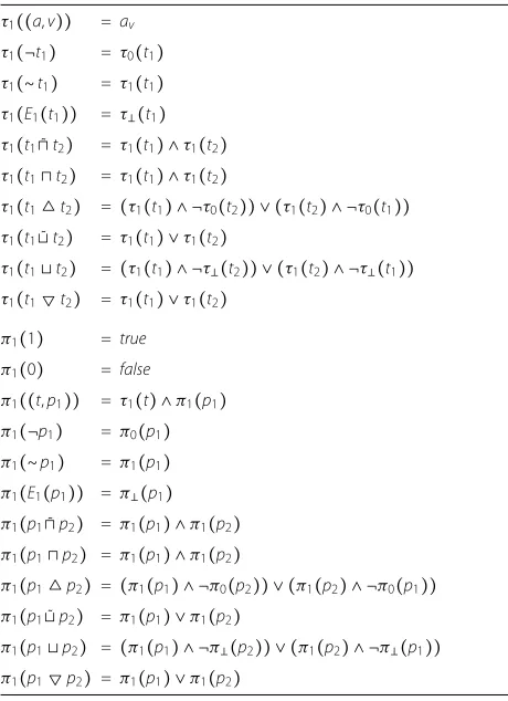
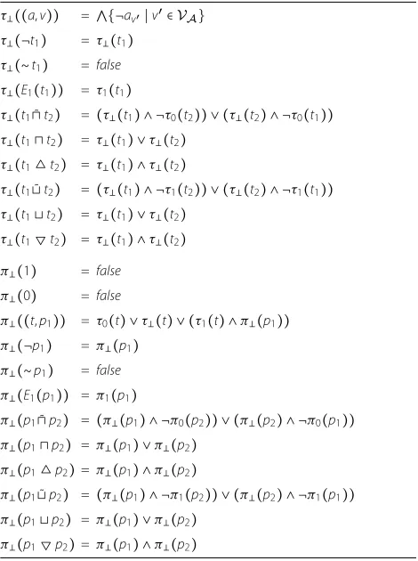
More specifically, each bd is a propositional formula representing a set of queries Qd ⊆ QA satisfying d = pB(q)wheneverq ∈ Qd. Hereafter, we writeτd(t)and πd(d) for the formulae representing decision d in the transformationτ(t)andπ(p), respectively. The transfor-mation rules forτ(for targets) andπ(for policies) given in Table2explain the construction of the propositional for-mula for decision 1 for all targets, (policy) constants and all (policy and target) operators of Table1. Tables3and4 present the transformation rules forτ (for targets) andπ (for policies) for decisions 0 and, respectively.
The correctness of the propositional formulaeτd(t)and πd(d)is stated by the following lemma.
Lemma 2For all q∈QA:
(a) I(q) ⊧τd(t)iffd=tT(q),
(b) I(q) ⊧πd(d)iffd=pB(q).
Example 3Let us reconsider policy p introduced in “Problem statement” section. By applying transformations τ andπin Tables2,3and4to p, we obtain (after minor simplification) the following propositional formulae:
π1(p) =natBE∧ ¬natNL π0(p) =natNL
π(p) = ¬natBE∧ ¬natNL
The corresponding BDDs are shown in Fig.2a (π1(p)),
Fig. 2b (π0(p)) and Fig.2c (π(p)). In the figures, solid
Table 2Transformation rules forτ(for targets) andπ(for policies) for decision 1
τ1((a,v)) = av
τ1(¬t1) = τ0(t1) τ1(∼t1) = τ1(t1) τ1(E1(t1)) = τ(t1) τ1(t1⊓˜t2) = τ1(t1) ∧τ1(t2) τ1(t1⊓t2) = τ1(t1) ∧τ1(t2)
τ1(t1△t2) = (τ1(t1) ∧ ¬τ0(t2)) ∨ (τ1(t2) ∧ ¬τ0(t1)) τ1(t1⊔˜t2) = τ1(t1) ∨τ1(t2)
τ1(t1⊔t2) = (τ1(t1) ∧ ¬τ(t2)) ∨ (τ1(t2) ∧ ¬τ(t1)) τ1(t1▽t2) = τ1(t1) ∨τ1(t2)
π1(1) = true
π1(0) = false
π1((t,p1)) = τ1(t) ∧π1(p1) π1(¬p1) = π0(p1) π1(∼p1) = π1(p1) π1(E1(p1)) = π(p1) π1(p1⊓˜p2) = π1(p1) ∧π1(p2) π1(p1⊓p2) = π1(p1) ∧π1(p2)
π1(p1△p2) = (π1(p1) ∧ ¬π0(p2)) ∨ (π1(p2) ∧ ¬π0(p1)) π1(p1⊔˜p2) = π1(p1) ∨π1(p2)
π1(p1⊔p2) = (π1(p1) ∧ ¬π(p2)) ∨ (π1(p2) ∧ ¬π(p1)) π1(p1▽p2) = π1(p1) ∨π1(p2)
whereas dashed arrows indicate that the attribute value is not present (i.e., the lo-edge); terminal nodes are repre-sented using a double line rectangle. These BDDs show that any query including attribute name-value pair(nat,NL) evaluates to0 and any query including attribute name-value pair(nat,BE)(and not(nat,NL)) evaluates to1; if both (nat,BE) and(nat,NL) are not present, the query evaluates to.
We also construct a propositional formulaS represent-ing the constrained query spaceQA∣C. This formula can be readily constructed by reusing transformationτ, since the constraint languageCA is essentially a subset of the target languageTA(see “Query constraints” section). The constrained query space can therefore be represented by the following propositional formula:
S= ⋀{τc1∣c∈C}
Example 4Figure2d shows the BDD encoding the con-strained query space for our example. Specifically, it is obtained by applying transformation τ to the cardinal-ity constraint in Example2(i.e., cardnat,3) in conjunction
with a query constraint imposing that individuals having an Austrian nationality cannot have dual nationality.
Table 3Transformation rules forτ(for targets) andπ(for policies) for decision 0
τ0((a,v)) = ¬av∧ ⋁{av′∣v′∈ VA}
τ0(¬t1) = τ1(t1) τ0(∼t1) = τ0(t1) ∨τ(t1) τ0(E1(t1)) = τ0(t1) τ0(t1⊓˜t2) = τ0(t1) ∨τ0(t2)
τ0(t1⊓t2) = (τ0(t1) ∧ ¬τ(t2)) ∨ (τ0(t2) ∧ ¬τ(t1)) τ0(t1△t2) = τ0(t1) ∨τ0(t2)
τ0(t1⊔˜t2) = τ0(t1) ∧τ0(t2) τ0(t1⊔t2) = τ0(t1) ∧τ0(t2)
τ0(t1▽t2) = (τ0(t1) ∧ ¬τ1(t2)) ∨ (τ0(t2) ∧ ¬τ1(t1))
π0(1) = false
π0(0) = true
π0((t,p1)) = τ1(t) ∧π0(p1) π0(¬p1) = π1(p1) π0(∼p1) = π0(p1) ∨π(p1) π0(E1(p1)) = π0(p1) π0(p1⊓˜p2) = π0(p1) ∨π0(p2)
π0(p1⊓p2) = (π0(p1) ∧ ¬π(p2)) ∨ (π0(p2) ∧ ¬π(p1)) π0(p1△p2) = π0(p1) ∨π0(p2)
π0(p1⊔˜p2) = π0(p1) ∧π0(2) π0(p1⊔p2) = π0(p1) ∧π0(p2)
π0(p1▽p2) = (π0(p1) ∧ ¬π1(p2)) ∨ (π0(p2) ∧ ¬π1(p1))
It is easy to observe in the BDD that queries including attribute name-value pair(nat,AT)and any other nation-alities are invalid (left part of Fig.2d); queries that contain four nationalities are invalid as well and thus all map to terminal vertex 0.
Policy evaluation
We now present our algorithm to compute the extended evaluation function⋅Eefficiently. The main idea is as fol-lows. Given a policy p, we construct a triple (e1,e0,e) of propositional formulae representing sets of queriesQ1,
Q0 and Q such that d ∈ pE(q) exactly when q ∈
Qd. As we do for the propositional formulae(b1,b0,b) representingpB, we represent these propositional for-mulae using (reduced) BDDs. For computing the triple of propositional formulae(e1,e0,e), we use the triple of propositional formulae(b1,b0,b)and the propositional formula S encoding the constrained query space QA∣C, along with a propositional formulaRencoding relation→∗ onQA∣C.
Table 4Transformation rules forτ(for targets) andπ(for policies) for decision
τ((a,v)) = ⋀{¬av′∣v′∈ VA}
τ(¬t1) = τ(t1) τ(∼t1) = false τ(E1(t1)) = τ1(t1)
τ(t1⊓˜t2) = (τ(t1) ∧ ¬τ0(t2)) ∨ (τ(t2) ∧ ¬τ0(t1)) τ(t1⊓t2) = τ(t1) ∨τ(t2)
τ(t1△t2) = τ(t1) ∧τ(t2)
τ(t1⊔˜t2) = (τ(t1) ∧ ¬τ1(t2)) ∨ (τ(t2) ∧ ¬τ1(t1)) τ(t1⊔t2) = τ(t1) ∨τ(t2)
τ(t1▽t2) = τ(t1) ∧τ(t2)
π(1) = false
π(0) = false
π((t,p1)) = τ0(t) ∨τ(t) ∨ (τ1(t) ∧π(p1)) π(¬p1) = π(p1)
π(∼p1) = false π(E1(p1)) = π1(p1)
π(p1⊓˜p2) = (π(p1) ∧ ¬π0(p2)) ∨ (π(p2) ∧ ¬π0(p1)) π(p1⊓p2) = π(p1) ∨π(p2)
π(p1△p2)= π(p1) ∧π(p2)
π(p1⊔˜p2) = (π(p1) ∧ ¬π1(p2)) ∨ (π(p2) ∧ ¬π1(p1)) π(p1⊔p2) = π(p1) ∨π(p2)
π(p1▽p2)= π(p1) ∧π(p2)
→∗ is in essence the subset relation, the proposition R encoding this relation is constructed by conjunctively composing the propositional formulae av ⇒ a′v. The correctness of this encoding is given by the following lemma.
Lemma 3Let q,q′ ∈ QA. Let I(q) denote the inter-pretation for Vars and I′(q′)the interpretation for Vars′, defined as I′(q′) (a′v) =true if and only if(a,v) ∈q′. We then have I(q) ∪I′(q′) ⊧ ⋀ {av⇒a′v∣av∈Vars}if and only if(q,q′) ∈→∗.
Note that we also need to ensure that only queries from the set represented bySare considered. We achieve this by strengthening the transition relation using the proposi-tional formulaS. This leads to the following propositional formula for the transition relationR:
S∧S[VarsA∶=Vars′A] ∧ ⋀ {av⇒a′v∣av∈VarsA}
The substitution notation we use in this formula is short-hand for replacing each unprimed variable by its primed counterpart in the propositional formula.
Using the triple(b1,b0,b), the constrained query space encoded bySand the transition relation encoded byR, we can compute a triple of propositional formulae(e1,e0,e) representing pE using a backwards reachability analy-sis. Since our transition relation Ris transitively closed, it essentially suffices to use R to compute all immedi-ate predecessors of b1,b0 and b. The computation of predecessors can be performed effectively on the level of BDDs using a standard encoding of the existential quantification over all primed variables. Fore1, this boils down to computing the (reduced) BDD for the following formula:
(S∧b1) ∨ ∃Vars′A.(R∧ (b1[VarsA∶=Vars′A]))
The computation ofe0andeproceeds analogously. We summarize the steps we take to compute the extended evaluation in Algorithm 1. The correctness of the algo-rithm is stated in the following theorem.
a
b
c
d
Algorithm 1Computing the extended evaluation for a policypand constrained query space(QA∣C,→).
1: procedureCOMPUTEEXTENDEDEVALUATION
2: (b1,b0,b) ∶= (π1(p),π0(p),π(p))
3: S∶= ⋀{τc1∣c∈C}
4: R∶=S∧S[VarsA∶=Vars′A] ∧ ⋀ {av⇒a′v∣av∈VarsA}
5: ford∈ {1, 0,}do
6: ed∶= (S∧bd) ∨ ∃Vars′A.(R∧ (bd[VarsA∶=Vars′A])) 7: end for
8: return(e1,e0,e)
9: end procedure
Theorem 4Procedure COMPUTEEXTENDEDEVALUA -TION computes, for a given policy p and a constrained query space (QA∣C,→), a triple(e1,e0,e)of BDDs
rep-resenting sets(Q1,Q0,Q) satisfying, for each q ∈ QA, q∈Qdiff q∈QA∣C∧d∈pE(q).
As we explained above, testing whether a truth-assignment to all variables makes a propositional formula true can be done in worst-case time O(∣Vars∣). As a consequence, the BDDs(e1,e0,e)that are computed by Algorithm 1 can be used to simply and efficiently evaluate a policypfor a concrete queryqusing the extended evalu-ation⋅E: for eachd∈ {1, 0,}, one evaluates at run-time whetherd∈pE(q)by inspecting BDDed, in worst-case timeO(∣Vars∣).
Example 5Figure 3 illustrates the BDDs (e1,e0,e)
encoding the extended evaluation of the policy in Exam-ple 4 augmented with the constrained query space in Fig.2d. The BDD in Fig.3a shows that a query will never be evaluated to1if it contains attribute name-value pairs (nat,NL) and (nat,AT). In fact, any query containing (nat,NL) is always evaluated to 0 as shown in Fig. 2b and a query containing (nat,AT) cannot be extended
as imposed by query constraints. The other paths in the BDD indicate that a query not including those attribute name-value pairs can potentially be evaluated to 1 as the query can be extended with attribute name-value pair (nat,BE)unless the query already includes three nation-alities (the maximum number of nationnation-alities allowed in our scenario). Similar observations hold for the other BDDs in Fig.3.
Case studies
In this section, we demonstrate our framework for the extended evaluation of ABAC policies using three real-world policies, namely the CONTINUE policy, the KMarket policy and the SAFAX policy. The framework has been implemented in Python using the dd library6 (v. 0.5.2).
The experiments were performed using a machine with 2.30GHz Intel Xeon processor and 16 GB of RAM.
Datasets
This section provides an overview of the policies used for our demonstration. The CONTINUEand SAFAX poli-cies are specified in XACML v2 (OASIS 2005) whereas the KMarket policy is expressed in XACML v3 (OASIS
a
b
c
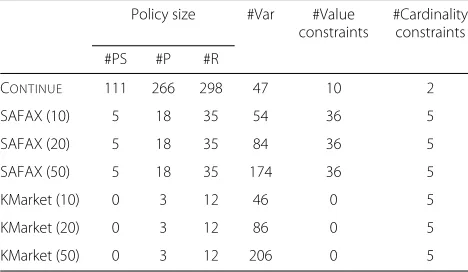
2013). XACML (both v2 and v3) has several common-alities with PTaCL; in particular, it has been shown in previous work (Morisset and Zannone2014) that XACML policies can be encoded in PTaCL. For the sake of space, we refer to Morisset and Zannone (2014) for the details of the encoding. A summary of the policies and datasets constructed from them is given in Table5. In the table, we report the size of the policies (in terms of number of policysets (#PS), policies (#P) and rules (#R)), the num-ber of variables used to encode the policy (#Var) and the number of cardinality and value constraints (i.e., query constraints excluding that two different attribute values can be present at the same time).
CONTINUE: CONTINUEis a conference manager system that supports the submission, review, discussion and noti-fication phases of conferences. The CONTINUE policy7 consists of 111 policysets that, in turn, consist of 266 cies comprising 298 rules. The target of policysets, poli-cies and rules are defined over 14 attributes ranging from the role of users (role) within the conference management system, the type of resource accessed (resource_class) and the action for which access is requested (action_type) to attributes used to characterize the existence of con-flicts of interest (isConflicted) and the status of the review process (isReviewContentInPlace, isPending, etc.). Some of these attributes are Boolean, whereas others, such as role and resource_class, take values from a more complex domain. In total, the union of the attribute domains for the CONTINUEpolicy consists of 47 attribute values.
Together with the policy, we specified 10 value con-straints. In particular, 9 constraints were used to enforce that Boolean attributes can be eithertrueorfalse.
The other value constraint was used to impose that subreviewers cannot be PC members as required by CONTINUE(Fisler et al.2005). Moreover, we defined two cardinality constraints to restrict the values that attributes resource_classandaction_typecan take as suggested in Fisler et al. (2005).
Table 5Overview of the datasets used for the experiments
Policy size #Var #Value #Cardinality constraints constraints #PS #P #R
CONTINUE 111 266 298 47 10 2
SAFAX (10) 5 18 35 54 36 5
SAFAX (20) 5 18 35 84 36 5
SAFAX (50) 5 18 35 174 36 5
KMarket (10) 0 3 12 46 0 5
KMarket (20) 0 3 12 86 0 5
KMarket (50) 0 3 12 206 0 5
SAFAX: SAFAX (2015) is an XACML-based framework that offers authorization as a service. SAFAX provides a web interface through which users can create, manage and configure their authorization services. The SAFAX policy is used to regulate the action users can perform on the web interface.
The SAFAX policy consists of 5 policysets, 18 policies and 35 rules. The target of these policy elements are built over 8 attributes ranging from the group(s) a user belongs to (group), the type of object to be accessed (type) and the action to be performed on the object (action) to the num-ber of objects a user has already created (count-project, count-demo, count-ppdp) and the relation of the user with the object (isowner, match_project). The last two attributes are Boolean, whereas the others have a more complex domain. In particular, three attributes range over integer numbers. To test the scalability of our approach, we varied the size of the domain of these attributes. In par-ticular, we generated three datasets – SAFAX (10), SAFAX (20) and SAFAX (50) – where the number in paren-theses represents the size of the domain of numerical attributes.
We also defined a number of query constraints that reflect the functioning of the system. Besides introducing constraints for Boolean attributes and cardinality con-straints for numerical attributes, we restricted the number of object types and actions that can occur in a request. This is motivated by the fact that, in SAFAX, an object can have only one type and access requests are triggered to determine whenever a user attempts to perform an action. Moreover, certain actions can be performed only on cer-tain types of objects. We modeled these domain require-ments using value constraints. We also defined constraints to restrict the groups a user can belong to simultaneously. Users should register to SAFAX to use the web applica-tion and can be assigned to multiple groups. Nonetheless, SAFAX also provides a guest account (with limited func-tionalities) that allows the use of the application without registration. Guest users are assigned to a special group that is incompatible with every other group. We cap-tured this requirement using value constraints. In total, we complemented the policy with 36 value constraints and 5 cardinality constraints.
andamount-liquor). The last four attributes range over the integers. Similarly to what done for the SAFAX pol-icy, we varied the size of the domain of these attributes. In particular, we generated three datasets – KMarket (10), KMarket (20) and KMarket (50) – where the number in parentheses represents the size of the domain of numer-ical attributes. We also defined cardinality constraints for numerical attributes and for the number of groups a user belongs to. The latter is motivated by the fact that a user can have only one type of subscription. In total, we complemented the policy with 5 cardinality constraints.
Evaluation
This section presents an evaluation of our framework using the CONTINUE, SAFAX and KMarket policies. First, we analyze the BDDs obtained using the extended evalua-tion funcevalua-tion⋅Eand its feasibility in real scenarios. Then, we evaluate the query evaluation time using a BDD repre-sentation of the extended evaluation and compare it with a SAT-based approach. Moreover, we investigate the use of attribute value power for an understanding of the impact of attributes on the decision making process. Finally, we present lessons learned from our experiments and discuss the limitations of the approach.
Analysis of extended evaluation function⋅E: For each dataset, Table 6 shows the size of the BDDs obtained using the simplified evaluation function ⋅B presented in “ABAC evaluation” section, and the size of the BDDs obtained using the extended evaluation function⋅Ewith
and without constraints. In particular, for each BDD, the table reports the number of vertices and the depth of the BDD. The depth of BDDs is particularly important as it affects policy evaluation (see “Efficient extended evalu-ation computevalu-ation” section). Table7 reports the size of the BDDs encoding the constrained query space for the datasets, which represent the set of valid queries (i.e., the queries that satisfy the constraints) along with the number of valid queries. This latter information provides an indication of the size of the constrained query space. Moreover, the table reports the percentage of queries that evaluate to 1, 0 andfor⋅Band⋅E. One can observe that, for⋅E, the sum of percentages is greater than 100%. Recall from “Preliminaries” section that ⋅E is defined overD8= ℘({1, 0,}).
The reported statistics were obtained after applying the garbage collection and reordering functions provided by the dd library. The garbage collector function deletes unreferenced nodes. Reordering is used to change the variable order to reduce the size of the BDD represen-tation. In particular, it uses Rudell’s sifting algorithm (1993), a widely used heuristics for dynamic reordering, to search for a better (fixed) order of variables compared the one currently used. Note that the reordering function is nondeterministic in the sense that it can return differ-ent orders of variables for the same input set of BDDs. This explains the differences in the number of nodes between the BDDs encoding the simplified evaluation of the SAFAX policy (top-left block of Table6)9.
In Table6(top-right block), we can observe that, when constraints are not considered, the BDDs encoding the
Table 6Overview of the BDDs encoding the simplified⋅Band extended⋅eevaluation with/without constraints
Simplified⋅B Extended⋅e
BDD1 BDD0 BDD BDD1 BDD0 BDD
#Vertex Depth #Vertex Depth #Vertex Depth #Vertex Depth #Vertex Depth #Vertex Depth
No constraints CONTINUE 1085 31 496 29 579 29 1 0 147 24 579 29
SAFAX (10) 347 24 370 24 7 6 1 0 430 24 7 6
SAFAX (20) 369 24 407 24 7 6 1 0 450 24 7 6
SAFAX (50) 343 24 366 24 7 6 1 0 427 24 7 6
KMarket (10) 38 15 38 15 4 3 37 15 1 0 4 3
KMarket (20) 87 36 87 36 4 3 86 36 1 0 4 3
KMarket (50) 326 125 326 125 4 3 325 125 1 0 4 3
Constraints CONTINUE 1156 46 510 46 846 46 594 44 672 46 830 46
SAFAX (10) 513 54 455 54 108 54 255 54 497 54 108 54
SAFAX (20) 949 84 920 84 188 84 375 84 762 84 188 84
SAFAX (50) 1587 174 1551 174 428 174 735 174 1540 174 428 174
KMarket (10) 207 46 246 46 76 43 206 46 137 43 76 43
KMarket (20) 408 86 510 86 156 83 407 86 277 83 156 83
Table 7BDD encoding constrained query space and percentage of queries that evaluate 1, 0,for⋅Band⋅E
#Vertex Depth #Queries Simplified⋅B Extended⋅E
BDDD1 BDD0 BDD BDD1 BDDD0 BDD
CONTINUE 63 44 134,631,720 20.09% 32.28% 47.52% 59.10% 41.48% 47.52%
SAFAX (10) 128 54 7,331,148 55.43% 28.39% 16.18% 97.10% 41.87% 16.18%
SAFAX (20) 188 84 51,009,588 55.36% 28.49% 16.18% 97.06% 43.03% 16.18% SAFAX (50) 368 174 730,641,708 55.27% 28.55% 16.18% 97.04% 42.14% 16.18%
KMarket (10) 77 43 468,512 26.41% 48.59% 25.00% 43.15% 90.08% 25.00%
KMarket (20) 157 83 6,223,392 20.03% 54.97% 25.00% 34.09% 92.35% 25.00% KMarket (50) 397 203 216,486,432 6.48% 68.52% 25.00% 11.18% 98.70% 25.00%
extended evaluation of the CONTINUEand SAFAX poli-cies for decision 1 and the extended evaluation of the KMarket policy for decision 0 consist of only one ver-tex. This vertex is the terminal vertex true, indicating that all queries can be potentially evaluated to 1 for the CONTINUEand SAFAX policies and to 0 for the KMar-ket policy. This is due to how these policies are defined. For instance, in the CONTINUEpolicy positive authoriza-tions have a higher priority than negative authorizaauthoriza-tions, i.e. all XACML policy elements are combined using the first-applicable combining algorithm and Permit rules always occur at the top, thus yielding permit whenever they are applicable. On the other hand, the SAFAX pol-icy specifies positive authorizations and employs Deny rules only as default rules. Similarly, the KMarket pol-icy specifies negative authorizations and employsPermit rules only as default rules. Thus, if all attribute values are provided in the query, the CONTINUE and SAFAX policies evaluate 1 and the KMarket policy evaluates 0. This demonstrates the importance of constraints. By look-ing at Table 7, we can observe that only 59% of queries could actually yield decision 1 for the CONTINUEpolicy and 97% for the SAFAX policy. We can also observe that the percentage of queries that evaluate 0 for the KMar-ket policy ranges between 90% (KMarKMar-ket (10)) and 98.70% (KMarket (50)). Thus, neglecting constraints can result in misleading decisions.
We can also observe from Table6that the BDDs encod-ing the simplified evaluation and the extended evaluation without constraints (top-left and top-right blocks, resp.) for are the same. This is expected as the applicability of both the CONTINUE, SAFAX and KMarket policies is monotonic; if they apply to a query, they also apply to all queries that can be constructed from it. Thus, it is not possible that a query evaluates toaccording to⋅E but not according to ⋅E. We can also observe that, for the SAFAX and KMarket policies, these BDDs are rela-tive small (7 nodes and depth equal to 6 for SAFAX, and 4 nodes and depth equal to 3 for KMarket) and, from Table7, that they cover about 16% and 25% of the query
space, respectively. This is due to the use of default rules mentioned above. Actually, these rules map most of the queries for which a positive authorization is not specified to 0 for SAFAX; similarly for KMarket, most of the queries for which a negative authorization is not specified are mapped to 1.
As discussed in “Efficient extended evaluation computa-tion” section, the depth of a BDD is upper bounded by the number of variables. We can observe in Table6 (bottom-left and bottom-right blocks) that, for the SAFAX policy with constraints, the depth of BDDs is exactly equal to the number of variables. This is due to the fact that the constraints defined for this policy involve all attribute values.
This is also visible by observing in Table5that the depth of the BDDs representing the constrained query space is equal to the number of variables, indicating that all variables are needed to determine the validity of queries.
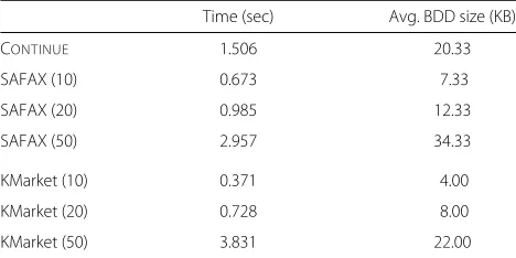
Feasibility of extended evaluation function ⋅E: To assess the feasibility of the approach, we considered the time needed to generate the BDDs encoding the extended evaluation of the CONTINUE and SAFAX policies along with the corresponding query constraints and the mem-ory required to store the generated BDDs. Table8reports
Table 8Time needed to construct the BDDs encoding the extended evaluation on the constrained query space and average BDD size
Time (sec) Avg. BDD size (KB)
CONTINUE 1.506 20.33
SAFAX (10) 0.673 7.33
SAFAX (20) 0.985 12.33
SAFAX (50) 2.957 34.33
KMarket (10) 0.371 4.00
KMarket (20) 0.728 8.00
the time required to generate the BDDs encoding the extended evaluation on the constrained query space. From the table, we can observe that the construction of BDDs for the CONTINUE policy required about 1.5s, whereas less than one second was required for the SAFAX (10), SAFAX (20), KMarket (10) and KMarket (20) datasets; SAFAX (50) required slightly less than 3 s and KMar-ket (50) required less than 4 s.
To estimate the memory required to store the generated BDDs, we exploited the functionalities of theddlibrary.
In particular, theddlibrary makes it possible to dump a BDD to a pickle file.
The average size of the dump files is reported in Table8. These results suggest that the precomputed BDDs can be stored and evaluated in resource-constrained devices, like IoT devices, to determine whether a user is allowed to access a device’s resources.
Query Evaluation Time: The BDDs constructed by our algorithm can be used straightforwardly to compute the decision for a concrete query. In essence, each BDD is no more than a large, nestedif-then-elseclause. Computing the decision for a concrete query thus amounts to evalu-ating a number of elementary Boolean conditions. Table9 provides the minimal, mean and maximal time (in sec-onds) it takes to compute the decision for a query for all seven datasets we considered in this paper. The timings were obtained by generating 100 (valid) queries.
We compare and contrast our BDD approach to a SAT approach for computing the extended decision; the approach is similar to that of Turkmen et al. (2017). Given the similarities with the BDD approach, we only sketch how SAT solving can be used to compute the extended decision. Using the encodingsτ andπ, we can construct a formulaφ1encoding all valid queries that evaluate to 1. For a concrete queryq, the formulaψ1used to compute whether 1∈pE(q), is then obtained by adding the clause
⋀{av ∣ (a,v) ∈ q}as a conjunction toφ1, ensuring that we only consider queries reachable fromq. Note thatψ1is
Table 9Time (in seconds) needed to compute the decision for a concrete query using BDDs and using SAT formulae; the minimal, mean and maximal time are taken from a sample of 100 valid queries
BDD SAT
min mean max min mean max
CONTINUE 0.0001 0.0002 0.0003 0.0370 0.0419 0.0483
SAFAX (10) 0.0001 0.0002 0.0004 0.0341 0.0383 0.0487 SAFAX (20) 0.0002 0.0004 0.0005 0.0581 0.0652 0.0727 SAFAX (50) 0.0005 0.0007 0.0009 0.2140 0.2298 0.2522 KMarket (10) 0.0001 0.0001 0.0002 0.0241 0.0268 0.0388 KMarket (20) 0.0001 0.0002 0.0003 0.0579 0.0687 0.0817 KMarket (50) 0.0002 0.0003 0.0004 0.2840 0.3011 0.3247
satisfiable if and only if 1∈pE(q). The formulaeψ0and ψare constructed analogously.
The timings reported on in Table9are obtained using the CVC4 solver (Barrett et al.2011). As far as the query evaluation time is concerned, BDDs clearly outperform the SAT approach. However, there may be cases in which a SAT-like approach may be more suited; e.g. when consid-ering attributes ranging over an infinite set of values, one may use SMT solvers to deal with the infinite domains.
Attribute Value Power: Thanks to the BDD encoding, it is relatively straightforward to compute the power of attribute values. Given a decisiondand an attribute name-value pair (a,v), the power can be computed by first computing the set of queries
Qda,v= (¬bd∧ (bd[av∶=true]) ∧S∧S[av∶=true])
wherebdis the BDD for the simplified evaluation andSis the BDD encoding the constrained query space.Qda,v cor-responds to all queriesqsuch that(q,(a,v))is a critical
pair. It follows thatPda,v= ∣Qda,v∣.∣∑(a′,v′)Qda′,v′∣ −1
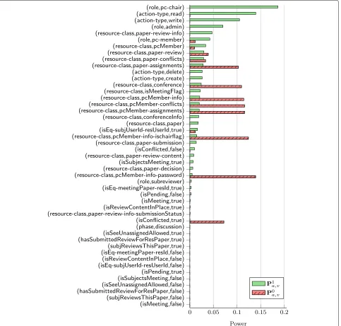
. Figure4displays the power of all attribute values for the CONTINUEpolicy. We can observe that the power is rel-atively distributed, with only three attribute values with a power higher than 0.10 for decision 1 (including role PC Chair, which is a good indicator of the importance of such an attribute value). There is a notable propor-tion of attributes with non-null power for either decision, although some attribute values (the bottom 9 on Fig.4) have a null power for both decisions.
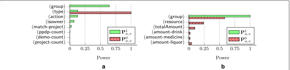
On the other hand, the power distribution for SAFAX (10) and KMarket (10), presented in Fig.5a and b (where, for the sake of presentation, we aggregate the power for all values for each attribute), respectively, are much less balanced. Indeed, for SAFAX there is a small number of attribute with non-null power for 0, which is consistent with the use of defaultDenypolicies. On the other hand, many attribute values have non-null power for decision 1, indicating that they can trigger decision 1 by adding them. KMarket adopts an opposite power profile behavior, with a small number of attribute values with a non-null power for 1, which is consistent with the use of defaultPermit policies.
Although there is no right or wrong power profile, the power analysis can help a policy designer to understand which attribute values are the most critical. For instance, in the case of SAFAX, as long as thetypeattribute is fully controlled (i.e., an attacker cannot hide the value for that attribute), we know no attribute hiding attack is possible.
Discussion
Fig. 4Power distribution for the CONTINUEpolicy: the plain green bar indicate the power for the decision 1 for each attribute value, while the patterned red bars indicate the power for the decision 0
scenarios. Moreover, we showed in Morisset et al. (2018) that the extended evaluation function ⋅E provides a more accurate evaluation of ABAC policies compared to standard evaluation function⋅p.
Nonetheless, our evaluation reveals that query con-straints have a significant impact on the extended evalu-ation function⋅E. On the one hand, query constraints improve the accuracy of policy evaluation by removing queries that cannot occur in practice. On the other hand, they affect the size of the BDDs representing policy evalu-ation because invalid queries have to be explicitly encoded in the BDDs. This is particularly the case for the SAFAX
policy, where the depth of the obtained BDDs is equal to the number of variables used for the encoding of the pol-icy, thus representing the worst case scenario. This result is due to the fact that domain constraints involve all vari-ables used for the encoding of the policy, indicating that all attribute values are needed to determine the validity of queries.