On the coupling of local 3D solutions and global 2D shell theory in structural mechanics

R E S E A R C H A R T I C L E

Open Access

On the coupling of local 3D solutions

and global 2D shell theory in structural

mechanics

Giacomo Quaranta

, Mustapha Ziane

, Fatima Daim

, Emmanuelle Abisset-Chavanne

,

Jean-Louis Duval

and Francisco Chinesta

*_{Correspondence:}

[email protected] 2_{PIMM, ENSAM ParisTech ESI}

GROUP Chair on Advanced Modeling and Simulation of Manufacturing Processes, 151 Boulevard de l’Hopital, 75013 Paris, France

Full list of author information is available at the end of the article

Abstract

Most of mechanical systems and complex structures exhibit plate and shell

components. Therefore, 2D simulation, based on plate and shell theory, appears as an appealing choice in structural analysis as it allows reducing the computational complexity. Nevertheless, this 2D framework fails for capturing rich physics compromising the usual hypotheses considered when deriving standard plate and shell theories. To circumvent, or at least alleviate this issue, authors proposed in their former works an in-plane-out-of-plane separated representation able to capture rich 3D behaviors while keeping the computational complexity of 2D simulations. However, that procedure it was revealed to be too intrusive for being introduced into existing commercial softwares. Moreover, experience indicated that such enriched descriptions are only compulsory locally, in some regions or structure components. In the present paper we propose an enrichment procedure able to address 3D local behaviors, preserving the direct minimally-invasive coupling with existing plate and shell discretizations. The proposed strategy will be extended to inelastic behaviors and structural dynamics.

Keywords: Plate and shells theories, In-plane-out-of-plane separated representations, PGD, Dynamics

Introduction

Many mechanical systems and complex structures involve plate and shell parts or com-ponents whose main particularity is having a characteristic dimension (the one related to the thickness) much lower than the other ones (in-plane dimensions). In order to analyse such structures, beam, plate and shell theories have been developed in solid mechan-ics [1,2] and extended later to many other physics, like flows in narrow gaps, thermal or electromagnetic problems in laminates, among many others. In these theories the introduction of appropriate kinematic and mechanic hypotheses on the evolution of the solution through the thickness of the plate (shell) allows the reduction of the general 3D mechanical problem to a 2D one involving the in-plane coordinates.

However, in many cases, when addressing complex coupled physics, inelastic behaviors or any other exhibiting localization, the validity of hypotheses able to reduce models from 3D to 2D becomes doubtful and consequently in order to ensure accurate results

©The Author(s) 2019. This article is distributed under the terms of the Creative Commons Attribution 4.0 International License (http://creativecommons.org/licenses/by/4.0/), which permits unrestricted use, distribution, and reproduction in any medium, provided you give appropriate credit to the original author(s) and the source, provide a link to the Creative Commons license, and indicate if changes were made.

3D discretizations seem compulsory. However mesh-based solutions of models defined in such degenerated domains is a challenging issue because the resulting meshes usually involve too many degrees of freedom, where the mesh size is almost determined by the domain thickness and the material and/or solution details to be represented. In order to alleviate the associated computational complexity in [3] authors proposed computing the fully 3D solution employing an in-plane-out-of-plane separated representation whose computational complexity remains the one characteristic of 2D plate or shell simulations, using the proper generalized decomposition-PGD-method [4].

However the proposed in-plane-out-of-plane separated representation appears to be too intrusive to be implemented in structural mechanics commercial software that gen-erally propose different plate and shell finite elements, even in the case of multilayered composites plates or shells. For this reason in this work we propose a minimally-intrusive method which allows integrating fully 3D local descriptions in plate or shell models imple-mented in any software, without affecting its computational complexity that remains the one related to standard 2D analyses. For that purpose, two different enrichment routes will be considered, the first based on the use of that separated representation and the sec-ond on a simple csec-ondensation. The former methodology allows for very fine 3D enriched descriptions while the last is particularly well adapted to address inelastic and dynamical behaviors.

Elastostatic problem definition

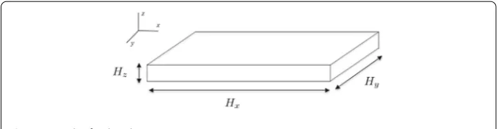
We consider the linear elastostatic problem defined in the plate domain depicted in Fig.1, = xy ×z, withxy = [0, Hx]×[0, Hy] andz = [0, Hz] in which the thickness (out-of-plane) dimension is much lower than the other ones, i.e.HzHx, Hy.

The linear elastic behavior relating the Cauchy’s stress σ and the strain ε tensors reads

σ=Cε, (1)

whereCis the Hooke’s fourth order tensor. The relation between strainεand displace-mentu(with componentsu=(u, v, w)) writes

ε= ∇su=Gu, (2)

where G = ∇s• = 1₂(∇ • +∇T•) is the symmetric gradient operator. Considering an homogeneous and isotropic material and using the Voigt notation, the Hooke’s tensor can be written as

C= E (1+ν)(1−2ν)

⎡ ⎢ ⎢ ⎢ ⎢ ⎢ ⎢ ⎢ ⎢ ⎣

1−ν ν ν 0 0 0

ν 1−ν ν 0 0 0 ν ν 1−ν 0 0 0 0 0 0 (1−₂2ν) 0 0 0 0 0 0 (1−₂2ν) 0

0 0 0 0 0 (1−₂2ν)

⎤ ⎥ ⎥ ⎥ ⎥ ⎥ ⎥ ⎥ ⎥ ⎦

. (3)

In absence of volumetric body forces, the displacement field evolutionu(x) forx∈is described by the linear momentum balance equation

∇ ·σ=0. (4)

The domain boundary∂is partitioned into Dirichlet,D, and Neumann,N, bound-aries, where displacementugand tractionsTare enforced respectively.

The problem weak form associated to the strong form (4) lies in looking for the dis-placement fieldu verifying the Dirichlet boundary conditions such that the weak form

ε(u

∗_{)·(Cε(u))dx=}

N

u∗·Tdx (5)

fulfills for any test functionu∗, with the trial and test fields defined in appropriate func-tional spaces.

In this type of domains, plate theory is usually used in order to reduce the general 3D mechanical problem to a 2D one involving the in-plane coordinates only. Two kinds of theories exist: the thin plate theory proposed by Kirchoff [5] which establishes that the normal remains straight and orthogonal to the middle plane after deformation and the thick plate theory proposed by Reissner [6] and Mindlin [7] which assumes that normals remain straight, but not necessarily orthogonal to the middle plane after deformation.

In both theories the middle plane is taken as the reference plane (z=0) for deriving the plane kinematic equations. In this work, we consider the Reissner–Mindlin theory whose fundamental hypotheses are the following: (i) on the middle plane (z = 0) the in-plane displacements vanish, i.e.u(x, y, z=0)=v(x, y, z=0)=0 that implies that points located in the middle-plane only moves vertically; (iii) the plate thickness remains unchanged; (iv) the plane stress assumption remains valid, i.e.σzz=0 and (v) a straight line normal to the undeformed middle plane remains straight but not necessarily orthogonal to the middle plane after deformation.

From these assumptions the displacement field can be written as:

⎧ ⎪ ⎨ ⎪ ⎩

u(x, y, z)= −zθx(x, y) v(x, y, z)= −zθy(x, y) w(x, y, z)=w(x, y)

(6)

wherewis the vertical displacement (deflection) of the points on the middle plane and the rotationsθxandθycoincide with the angles followed by the normal vectors contained in the planesxzandyzrespectively in their motions.

We define the generalized displacement vectorˆu

ˆu=[θx,θy, w]T (7)

Injecting plate theory assumptions into the 3D elastostatic problem weak form, Eq. (5) reduces to the following 2D formulation [1]

xy

ˆ

ε(ˆu∗)·Cˆˆε(ˆu)dx=

∂Nxy

ˆu∗_·Tˆ_{dx, (8)}

whose standard finite element discretization leads to

KU=F (9)

where for notational simplicity the hat symbol (ˆ•) is omitted. In the previous expression (9),Kis the stiffness matrix andUandFare the vector of the generalized displacements and forces, the former containing nodal rotations and deflections and the last the dual quantities: the nodal moments and vertical nodal forces. The 3D displacement field can be then recovered by using the relations (6).

In many cases, the complexity of the solution makes impossible the introduction of pertinent hypotheses for reducing the dimensionality of the model from 3D to 2D. In that case a fully 3D descriptions seems compulsory, and the in-plane-out-of-plane separated representations become particularly suitable.

In-plane-out-of-plane separated representation

The in-plane-out-of-plane separated representation was proposed in [3] and applied to efficiently solve 3D elastic problems in plate geometries. The elastic problem was defined in a plate domain= xy×zwith (x, y)∈xy,xy ⊂ R2andz ∈z,z⊂ R. The separated representation of the displacement fieldu = (u, v, w) consists in a finite sum decomposition onNterms, each one of them consisting in the product of two unknown functions, one depending on the in-plane coordinates (x, y) and one on the out-of-plane coordinatez, i.e.:

u(x, y, z)=

⎛ ⎜ ⎜ ⎜ ⎝

u(x, y, z)

v(x, y, z)

w(x, y, z)

⎞ ⎟ ⎟ ⎟

⎠≈

N

i=1

⎛ ⎜ ⎜ ⎜ ⎝

ui

xy(x, y)·uiz(z)

vi_xy(x, y)·vi_z(z)

wi_xy(x, y)·w_zi(z)

⎞ ⎟ ⎟ ⎟

⎠. (10)

Expression (10) can be written in a more compact form by using the Hadamard (component-to-component) product:

u(x, y, z)≈ N

i=1

Ui

xy(x, y)◦Uzi(z). (11)

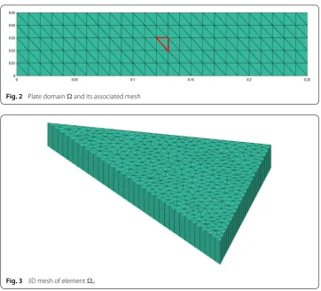
Fig. 2 Plate domainand its associated mesh

Fig. 3 3D mesh of element_e

However the proposed in-plane-out-of-plane separated representation remains too intrusive to be implemented in structural mechanics commercial softwares that instead, propose a variety of plate and shell elements.

For this reason in the next section we propose a method which allows enriching standard plate and shell discretizations while limiting intrusivity.

Enriched formulations

PGD-based enriched elements

We assume the 2D mesh defined on the middle plane of a plate geometry, depicted in Fig.

2. Our goal here is to address one element of the mesh, for example the one whose bound-ary is highlighted in red and that is noted bye, by using a fully 3D description in order to extract its homogenized 9×9 element stiffness matrix corresponding toe, and therefore fully compatible with the plate kinematics enforced on the element boundary∂e.

For that purpose,eis 3D resolved using the PGD-based in plane-out-of-plane sep-arated representation while a kinematics compatible with the plate kinematics (6) is enforced on the element boundary. All the other elements in depicted in Fig.2are described using the standard plate theory, the only 3D resolved is just theewhose 3D mesh is depicted in Fig.3.

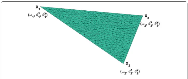
Fig. 4 Nodal degrees of freedom defining the kinematics on∂e ⎧ ⎪ ⎪ ⎪ ⎪ ⎪ ⎪ ⎪ ⎪ ⎪ ⎪ ⎪ ⎪ ⎪ ⎨ ⎪ ⎪ ⎪ ⎪ ⎪ ⎪ ⎪ ⎪ ⎪ ⎪ ⎪ ⎪ ⎪ ⎩

ue,1_xy(x, y)=θ₁xN1(x, y)+θ2xN2(x, y)+θ3xN3(x, y) ve,1

xy(x, y)=θ y

1N1(x, y)+θ y

2N2(x, y)+θ y 3N3(x, y) we,1_xy(x, y)=ω1N1(x, y)+ω2N2(x, y)+ω3N3(x, y) ue,1z (z)= −z

ve,1z (z)= −z

we,1z (z)=1

(12)

whereN1(x, y),N2(x, y) andN3(x, y) are the shape functions related to the 2D linear trian-gular elemente, and

Ue=(ω1,θ₁x,θ₁y,ω2,θ₂x,θ₂y,ω3,θ₃x,θ₃y) (13)

are the nine degrees of freedom associated to its three vertices, depicted in Fig.4. Once the first mode has been imposed the following modes are constructed as described in section while ensuring that they vanish on the element boundary∂e. The last condi-tion can be enforced by using the so-called bubble funccondi-tion that results from the product of the three triangle shape functionsB(x, y)=N1(x, y)N2(x, y)N3(x, y) (even if other alter-natives exist for that purpose [10]), i.e.∀i>1

⎧ ⎪ ⎪ ⎪ ⎪ ⎪ ⎪ ⎪ ⎪ ⎪ ⎪ ⎪ ⎪ ⎪ ⎨ ⎪ ⎪ ⎪ ⎪ ⎪ ⎪ ⎪ ⎪ ⎪ ⎪ ⎪ ⎪ ⎪ ⎩

ue,i_xy(x, y)=B(x, y)Pi_x(x, y)

ve,i

xy(x, y)=B(x, y)Pyi(x, y)

we,i_xy(x, y)=B(x, y)Pi_z(x, y)

ue,iz (z)=Txi(z)

ve,iz (z)=Tyi(z)

we,iz (z)=Tzi(z)

(14)

In order to extract the effective enriched 9×9 element stiffnessKe_{(related to element} e) to be assembled into the global stiffness matrix involved in the algebraic system (9), we consider the element average

• =

e

•dx, (15)

from which the element elastic energyUebecomes

Ue₌eT_σe₌eT_Ce_{. (16)}

Now, with the strain defined from (2) we assume the existence of a localization tensor

Lsuch that

ue_=LUe_{, (17)}

that using Eq. (2) results

e_{= ∇}

sue=GLUe, (18)

whereUe, as previously indicated, represents the plate generalized displacement degrees of freedom defined in (13).

Thus, the components of the localization tensor result from the elastic problem solution ineby prescribing the canonical boundary displacements, i.e.Ue₁=(1,0,0,0,0,0,0,0,0),

Ue

2=(0,1,0,0,0,0,0,0,0), and so on, with nine associated 3D elastic problems solved by using the PGD-based in-plane-out-of-plane separated representation.

Then, by definingM=GLwe obtain

Ue_=UeT

MT_CMUe_=UeT

MT_CMUe_{, (19)}

which allows defining the element stiffness matrixKe_as

Ke_=MT_{CM. (20)}

In order to check the procedure, the stiffness matrixKeobtained using the first mode of the displacement expansion is compared to that one corresponding to the plate kinematics. In that case, the resulting stiffness matrix was, as expected, the one related to standard plate theory.

Of course, when considering more modes in the separated representation of the 3D displacement field ue, the resulting stiffness matrixKe differs from the one associated to standard plate theory by including eventual 3D effects ignored in standard plate kine-matics. However, in that case the expression of the effective enriched stiffness matrix

Static condensation based enrichment

In this section, we consider an alternative procedure for computing the homogenized element stiffness matrix using static condensation [12].

We consider again the problem defined in the domainedepicted in Fig.3. The nodal degrees of freedom used for discretizing the displacement fieldue,Ue, can be decomposed in the ones related to internal nodesUe_i and the ones related to nodes located on∂e,Ue_b.

Thus, the standard 3D finite element formulation

Ke_Ue_=Fe_{, (21)}

with

Ke₌

Ke ii Keib Ke

biKebb

, (22)

can be expressed as

Ke ii Keib Ke

biKebb Ue

i Ue b

=

Fe i Fe b

. (23)

Now, by developing the first row of the previous system, the internal degrees of freedom can be expressed from the ones on the element border,

Ue i =Ke

−1

ii

Fe

i −KeibUeb

, (24)

that inserted in the second leads to

Ke

bbUeb=Fbe, (25)

with

Ke

bb=Kebb−KebiKe

−1

ii Keib (26)

Fe

b=Feb−KebiKe

−1

ii Fei. (27)

Now we enforce on the element border a kinematic compatible with the one of the plate theory, that is, the border nodal displacementsUe_bare expressed formUe[(the plate theory degrees of freedom defined at the triangle vertices as expressed in Eq. (13)], according to Eq. (6), relation that is expressed in matrix form fromUe

b=BUe. Thus, Eq. (25) can be rewritten as

Ke

bbBUe=Fbe, (28)

that premultiplying byBT (looking for the Galerkin based discrete system) results

BT_Ke

bbBUe=BTFbe, (29)

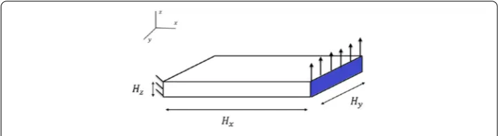
Fig. 5 Elastic problem defined in a plate domain

Table 1 Problem parameters

Hx: Length in thexdirection (mm) 250

Hy: Length in theydirection (mm) 50

Hz: Length in thezdirection (mm) 2

E: Young modulus (N/m2) 2·1011

ν: Poisson coefficient 0.25

Table 2 Parameters values used in the simulation

Nx(number of elements in the_xdirection): 25

Ny(number of elements in the_ydirection): 5

Nz(number of elements in the_zdirection): 11

˜

Ke_=BT_Ke

bbB (30)

˜

Fe_=BT_Fe_{. (31)}

Our numerical simulation allowed proving that the effective plate element stiffness matrix ˜Keobtained using the just described rationale based on the static condensation coincides with the one previously obtained by using the PGD-based separated represen-tationKe.

An additional advantage of this second route is the fact of deriving an expression for the effective plate nodal forces that will be advantageously considered when addressing inelastic and dynamic behaviors.

Numerical validation

We solve the elastic problem in the plate domain depicted in Fig.5 and compare the solutions obtained using 3D FEM, the standard plate theory and the enriched formulations considered in the previous section. The domain geometry=[0, Hx]×[0, Hy]×[0, Hz] is defined in Table1whereas Table2specifies the considered mesh.

On the domain right face (blue area in Fig. 5) a vertical traction is applied, T = (0,0,10000)N/m2_{whereas the displacement is prevented on the opposite face.}

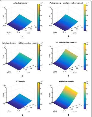
Figure6compares the different computed solutions. In that figure “3D solution” refers to the solution obtained using 3D elements according to the mesh specified in Table2. As reference solution we consider a 3D finite element solution using a much finer mesh (the one defined in Table3).

0 0.05 1 0.3 z (m) 10-4 2

All plate elements

y (m) 0.2 x (m) 3 0.1 0 0 0 0.5 1 1.5 2 2.5 10-4 a 0 0.05 1 0.3 z (m) 10-4 2

Plate elements + one homogenized element

y (m) 0.2 x (m) 3 0.1 0 0 0 0.5 1 1.5 2 2.5 10-4 b 0 0.05 1 0.3 10-4 z (m) 2

Half plate elements + half homogenized elements

y (m) 0.2 x (m) 3 0.1 0 0 0 0.5 1 1.5 2 2.5 10-4 c 0 0.05 1 0.3 10-4 z (m) 2

All homogenized elements

y (m) 0.2 x (m) 3 0.1 0 0 0 0.5 1 1.5 2 2.5 10-4 d 0 0.05 1 0.3 z (m) 10-4 2 3D solution y (m) 0.2 x (m) 3 0.1 0 0 0 0.5 1 1.5 2 2.5 10-4 e 0 0.05 1 0.3 10-4 z (m) 2 Reference solution y (m) 0.2 x (m) 3 0.1 0 0 0 0.5 1 1.5 2 2.5 10-4 f

Fig. 6 Displacement of the plate middle plane using plate theory (a), all plate theory elements except the

homogenized (enriched) element (b), half plate theory elements (the triangles of the mesh in Fig.2with the right angle on the bottom) and half homogenized (enriched) elements (the triangles of the mesh in Fig.2

with the right angle on the top) (c), all homogenized (enriched) elements (d), fully 3D FEM on a coarse mesh (e), fully 3D FEM on fine mesh (f)

It is important to note that even when all the element are enriched, the solution exhibits a gap with respect to the reference solution. This gap can be explained by the fact that despite of the valuable enrichments introduced at the elements level, at the elements boundaries standard plate kinematics is enforced with its consequent impact on the resulting kinematic that continue to be too constrained with respect to a fully 3D kine-matics.

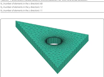
Table 3 Parameters values used in the simulation for the reference solution

Nx(number of elements in thexdirection): 60

Ny(number of elements in theydirection): 12

Nz(number of elements in thezdirection): 11

Fig. 7 Holed 3D triangular element and its associated mesh

later) but whose effects remain confined in the interior of that element (or patch) and when approaching to the element border the plate kinematic is accurate enough.

In the case here discussed plate theory and coarse 3D finite element solutions are closer one to the other, whereas the enriched one is the closest to the reference one (refined 3D finite element solution).

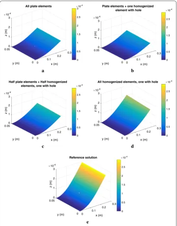
We consider the same problem as in the previous example but now we suppose that in the 3D element there is an hole as depicted in Fig.7(in the other elements we consider the enrichment presented before in absence of holes).

Here, there is clearly a double advantage in using the enrichment methodology. First, if the effect of the hole remains confined inside the element, vanishing when approaching the element boundary, the element enriched suffices and the plate meshing can be alleviated because the hole only exist for the element that will be accordingly enriched, but remains invisible at the plate level. On the other hand, its local 3D effects will be described very accurately.

Once the holed element stiffness matrixKeis computed using the procedure presented in the previous section, the problem is solved and the generalized displacement fieldUe can be extracted at the vertices of the holed triangle. Then the 3D solution inside the element can be easily computed by using (17). Figure8depicts different solutions. Even if e accounts the hole presence (the PGD and static condensation based enrichment proceed on a mesh that describe the hole presence), the plate mesh becomes unaltered.

As discussed, after solving the problem at the plate level, using the enriched stiffness matrices for the different elements, 3D fields can be reconstructed. Thus, Figs.9,10and

0 0.05 1 0.3 z (m) 10-4 2

All plate elements

y (m) 0.2 x (m) 3 0.1 0 0 0 0.5 1 1.5 2 2.5 310 -4 a 0 0.05 1 0.3 z (m) 10-4 2

Plate elements + one homogenized element with hole

y (m) 0.2 x (m) 3 0.1 0 0 0 0.5 1 1.5 2 2.5 10-4 b 0 0.05 1 0.3 10-4 z (m) 2

Half plate elements + Half homogenized elements, one with hole

y (m)

0.2

x (m) 3

0.1

0 0 0

0.5 1 1.5 2 2.5 10-4 c 0 0.05 1 0.3 10-4 z (m) 2

All homogenized elements, one with hole

y (m)

0.2

x (m) 3

0.1

0 0 0

0.5 1 1.5 2 2.5 10-4 d 0 0.05 1 0.3 10-4 z (m) 2 Reference solution y (m) 0.2 x (m) 3 0.1 0 0 0 0.5 1 1.5 2 2.5 10-4 e

Fig. 8 Displacement of the plate middle plane using plate theory (a), all plate theory elements except the

homogenized (enriched) holed element (b), half plates theory elements (the triangles of the mesh in Fig.2

with the right angle on the bottom) and half homogenized elements (the triangles of the mesh in Fig.2with the right angle on the top), one of them holed (c), all homogenized elements, one of them holed (d), fully 3D theory on the fine mesh (e)

that is neglected when using standard plate theory. Moreover, a parabolic evolution of the componentsσxzandσyzalong the domain thickness can be noticed in Fig.11.

Extension of the method to patches

-1 0.028 0

0.118

z (m)

10-3

xz (N/m 2

)

y (m)

0.026

x (m)

1

0.116

0.024 0.114

0 2 4 6 8

107

a

-1 0.028 0

0.118

z (m)

10-3

yz (N/m 2

)

y (m)

0.026

x (m)

1

0.116

0.024 0.114

-2 0 2 4 6

107

b

-1 0.028 0

0.118

z (m)

10-3

zz (N/m

2₎

y (m)

0.026

x (m)

1

0.116

0.024 0.114

-1 -0.5 0 0.5 1

107

c

Fig. 9 Out-of-plane components of the stress tensor around the hole

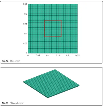
patch delimited by the red line in Fig.12,p, treat it using a 3D description by employing one of the two procedures previously presented (the PGD in-plane-out-of-plane separated representation or the static condensation procedure) and then construct the (3Nb)×(3Nb) patch stiffness matrix (being N_b the number of nodes in the border of the enriched patch). In the case here addressed numerically, the stiffness matrix size will be 84×84. In the construction procedure it is assumed that on the patch border the kinematic is the standard plate kinematic applied in the surrounding elements.

In the present case the generalized patch displacement reads

U=(θ₁x,θ₁y,ω1,θ₂x,θ₂y,ω2,. . .,θ_Nx

b,θ

y

Nb,ωNb), (32)

withNb=28. Figures12,13and14depict respectively the patch location, its 3D repre-sentations and its connection with the surrounding plate elements.

In the numerical validation we consider again the problem depicted in Fig.5, where the geometrical and mechanical properties are defined in Table4. On the right face (the blue area in Fig.5) a vertical traction is applied,T =(0,0,1100000)N/m2whereas on the opposite face the displacement is prevented.

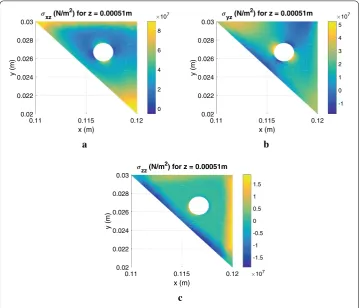
0.11 0.115 0.12 x (m) 0.02 0.022 0.024 0.026 0.028 0.03 y (m)

xz (N/m 2

) for z = 0.00051m

0 2 4 6 8 107 a b

0.11 0.115 0.12

x (m) 0.02 0.022 0.024 0.026 0.028 0.03 y (m)

yz (N/m 2

) for z = 0.00051m

-1 0 1 2 3 4 5 107

0.11 0.115 0.12

x (m) 0.02 0.022 0.024 0.026 0.028 0.03 y (m)

zz (N/m 2

) for z = 0.00051m

-1.5 -1 -0.5 0 0.5 1 1.5 107 c

Fig. 10 Out-of-plane components of the stress tensor on the planez=0.51 mm

0 2 4 6 8

xz (N/m 2

) 107

-1 -0.5 0 0.5 1 z (m)

10-3 xz of a point in hole border

a b

-10 -8 -6 -4 -2 0

yz (N/m 2

) 106

-1 -0.5 0 0.5 1 z (m)

10-3 yz of a point in hole border

Fig. 11 Out-of-plane components of the stress tensor through the domain thickness in the hole

neighborhood

solution has been computed using a mesh as fine as the one considered to describe the enriched solution at the patch level.

Fig. 12 Plate mesh

Fig. 13 3D patch mesh

one related to enriched elements where the kinematic constrains are applied to all the elements boundaries, its accuracy is superior.

Since it is not pretended that plates should be discretized using enriched super-elements, our main interest is adopting accurate descriptions of rich behaviors that could be assumed confined inside a region (our patch). This is the route retained for replacing 3D FEM discretization in regions exhibiting rich behaviors by enriched super-elements keeping its 2D computational complexity.

Extension of the method to plasticity

In this section we extend the method to problems in which plastic behavior can occur. In fact localized plasticity phenomena can occur in several situation, as in spot-welds during crash simulations.

In its general form the infinitesimal relation between the stress incrementdσand the elastic straindeincrement reads [13]

dσ=Cde=C(d−dp), (33)

Fig. 14 Patch discretization

Table 4 Model parameters

Hx: Length in thexdirection (mm) 250

Hy: Length in the_ydirection (mm) 250

Hz: Length in thezdirection (mm) 2

E: Young modulus (N/m2) 2 1011

ν: Poisson coefficient 0_.25

In plasticity yielding can occur only if the stresses satisfy a general yield criterion; in the considered examples, for the sake of simplicity, we use the Von Mises criterion [14], assuming perfect plasticity. Ignoring volumetric body forces, the weak form of the prob-lem, in its finite incremental form, associated to the strong form (4) lies in looking for the displacement field increment uverifying the Dirichlet boundary conditions, verifying

ε(u

∗_{)·(C( ( u)−} p_{( u)))dx=}

N

u∗_{· Tdx (34)}

for any test functionu∗in an appropriate functional space.

In order to solve the resulting nonlinear problem, various computational procedures have been proposed and extensively used, among them [15–22].

In this work we consider a simple implicit approach that at thenload step solves

ε(u

∗_)·C 1 n

dx=

N

0 0.01 0.02 0.3 z (m) 0.2 0.03

All plate elements

y (m) 0.2 x (m) 0.04 0.1 _0.1 0 0 0 0.005 0.01 0.015 0.02 0.025 0.03 a b c d 0 0.01 0.02 0.3 z (m) 0.2 0.03

Plate elements + one patch element

y (m) 0.2 x (m) 0.04 0.1 _0.1 0 0 0 0.005 0.01 0.015 0.02 0.025 0.03 0 0.01 0.02 0.3 z (m) 0.2 0.03

All patch elements

y (m) 0.2 x (m) 0.04 0.1 _0.1 0 0 0 0.005 0.01 0.015 0.02 0.025 0.03 0 0.01 0.02 0.3 z (m) 0.2 0.03 Reference solution y (m) 0.2 x (m) 0.04 0.1 _0.1 0 0 0 0.005 0.01 0.015 0.02 0.025 0.03

Fig. 15 Displacement using plate theory (a), all plate theory elements except the patch super-element (b),

all patches as depicted in Fig.16(c), fully 3D refined FEM (d)

Table 5 Coarse 3D FEM

Nx(number of elements in thexdirection): 21

Ny(number of elements in theydirection): 21

Nz(number of elements in thezdirection): 5

from 1_n, the stress increment 1_nσresults

1

nσ=C 1n (36)

that allows updating the stress

σ1

n=σn−1+ 1nσ, (37)

and from it computing the plastic strain increment 1

npusing well known procedures. Then, the stress is updated according to

σ1

n=σ1n−C 1np. (38)

Then, 2_nis calculated from

(u

∗_)·C 2 n

dx=

(u

∗_)·C 1 np

Table 6 Refined 3D FEM considered for defining the reference solution

Nx(number of elements in thexdirection): 63

Ny(number of elements in theydirection): 63

Nz(number of elements in thezdirection): 5

and the stress update from

σ2

n=σ1n+ 2nσ, (40)

and from it computing the plastic strain increment 2_npusing well known procedures. Then, the stress is updated according to

σ2

n=σ2n−C 2np. (41)

At iterationjthe problem to be solved reads

(u

∗_)·C j n

dx=

(u

∗_)·C j−1 n p

dx, (42)

where it can be noticed that the problem structure remains unaltered, with the left-hand member encountered when addressing elastic behaviors, the inelastic behavior appearing as a body force. Thus, the enrichment procedure based on the static condensation seems specially suitable.

For validating the proposed strategy we consider the same problem as in the previous section, sketched in Fig.5, with geometrical and mechanical properties specified in Table

4and the considered mesh defined in Table5. On the right face of the domain (blue area in Fig.5) a vertical traction is applied,T =(0,0,1100000)N/m2, and on the opposite face displacement is prevented. The considered uniaxial stress yield isσ0 = 250·106N/m2. Again, Fig.17depicts the usual different solutions. Again “all patch elements” refers to the case in which the domain is composed by the nine super-elements shown in Fig.16. The 3D reference solution has been computed using a mesh as fine as with the one used in the patch description (Table6). Again, the nine-patches solution is the most accurate (when compared with the reference solution).

Extension to structural dynamics

In this section we address structural dynamic, again ignoring body forces without loss of generality. Thus, the displacement field evolution u(x, t) in the domain and time intervalt∈I=(0, T] is described by the linear momentum balance equation

ρu¨(x, t)=divσ, (43)

whereρis the density (kg/m3).

Fig. 16 Super-element discretization

0 0.3

0.3 0.05

z (m)

0.2

All plate elements

y (m)

0.2

x (m)

0.1

0.1 _0.1

0 0

0 0.01 0.02 0.03 0.04 0.05 0.06 0.07 0.08 0.09

a b

c

0 0.3

0.3 0.05

z (m)

0.2

All patch elements

y (m)

0.2

x (m)

0.1

0.1 _0.1

0 0

0 0.01 0.02 0.03 0.04 0.05 0.06 0.07 0.08 0.09

0 0.3

0.3 0.05

z (m)

0.2

Reference solution

y (m)

0.2

x (m)

0.1

0.1

0.1 0 0

0 0.01 0.02 0.03 0.04 0.05 0.06 0.07 0.08 0.09

Fig. 17 Plate theory displacement (a), all patch elements according to Fig.16(b) and refined 3D FEM

(reference solution) (c)

In the elastic case the problem weak form associated with the strong form (43) results in looking for the displacement fielduverifying the initial and Dirichlet boundary conditions, and fulfilling

ρ

u

∗_·u¨dx+

ε(u

∗_{)·(Cε(u))dx=}

N

u∗_{·T(t)dx (44)}

Table 7 Model parameters

Hx: Length in thexdirection (m) 3

Hy: Length in theydirection (m) 3

Hz: Length in thezdirection (m) 0.1

E: Young modulus (N/m2) 2 1011

ν: Poisson coefficient 0.25

Table 8 Coarse FEM mesh

Nx(number of elements in the_xdirection): 21

Ny(number of elements in the_ydirection): 21

Nz(number of elements in the_zdirection): 5

Table 9 Refined FEM mesh considered for computing the reference solution

Nx(number of elements in the_xdirection): 63

Ny(number of elements in the_ydirection): 63

Nz(number of elements in the_zdirection): 5

The standard FEM space discretization reads

Ma(t)+Ku(t)=F(t), (45)

wherea(t) represents the acceleration. The time stepping consists in calculating the accel-eration and displacement at each time steptj₊1=(j+1) tfrom the ones existing at the previous time steptj=j t.

A widely considered choice consists of the Newmark method [23] in which the velocity and the displacement fields at timetj+1read

vj+1=vj+ t

(1−γ)aj+γaj+1

, (46)

and

uj+1=uj+ tvj+

t2 2

(1−2β)aj+2βaj+1

, (47)

so that at each time step the acceleration field can be obtained by solving the linear system

K∗aj+1=p∗j+1 (48)

where

K∗=M+β t2K (49)

and

p∗

j+1=Fj+1−Kuj− tKvj− t2

2 (1−2β)Kaj. (50)

Fig.

18

Elastic

displacement

using

p

late

theory,

n

ine-patches

and

3D

FEM

o

n

the

refined

mesh

at

four

d

ifferent

0 0.5 1 1.5 2 2.5 3 3.5 4 4.5 5

time (s) 104

-0.2 -0.15 -0.1 -0.05 0 0.05 0.1 0.15 0.2

vertical displacement (m)

Elasticity

Solution with plate elements Solution with patches 3D reference solution

Fig. 19 Vertical elastic displacement evolution in time at the right border

An enriched stiffness can be derived at the element or patch levels, where the use of the the procedure based on the condensation allows properly addressing the forcesp∗_j+1, and therefor combining dynamics and plasticity.

For evaluating the performances of the proposed enrichment procedure, we consider again the problem defined in Fig.5and Table7.

On the right face (the blue area in Fig.1) a vertical traction is enforced,T(t)=(0,0,4.1· 106sin(2πωt))N/m2, whereas on the opposite face displacement is prevented. Without loss of generality homogeneous initial conditionsu(x, t =0)=0 andv(x, t =0)=0 are assumed. Table8reports the considered coarse mesh whereas Table9defined the refined one from which the reference solution is calculated.

Figures18and19depict respectively the solutions computed using the different tech-niques at four different times and the vertical displacement time evolution at the right border. Figures20and21present similar results but in a case where plasticity takes place. Again the best solutions are the ones related to a nine-patches discretization for the reasons widely exposed before.

Conclusions

Fig.

20

Elasto-plastic

displacement

using

p

late

theory,

n

ine-patches

and

3D

FEM

o

n

the

refined

mesh

at

four

d

ifferent

0 0.5 1 1.5 2 2.5 3 3.5 4 4.5 5

time (s) 104

-1.5 -1 -0.5 0 0.5 1 1.5

vertical displacement (m)

Plasticity

Solution with plate elements Solution with patches 3D reference solution

Fig. 21 Vertical elasto-plastic displacement evolution in time at the right border

Authors’ contributions

All the authors participated in the definition of techniques and algorithms. G. Quaranta, developed moreover the simulation software, assisted by M. Ziane. All authors read and approved the final manuscript.

Author details

1_{ESI Group, Parc Icade, Immeuble le Seville, 3 bis, Saarinen, CP 50229, 94528 RUNGIS CEDEX, France,}2_{PIMM, ENSAM}

ParisTech ESI GROUP Chair on Advanced Modeling and Simulation of Manufacturing Processes, 151 Boulevard de l’Hopital, 75013 Paris, France.

Acknowledgements

This project has received funding from the European Union’s Horizon 2020 research and innovation programme under the Marie Skłodowska-Curie grant agreement No. 675919.

Competing interests

The authors declare that they have no competing interests.

Publisher’s Note

Springer Nature remains neutral with regard to jurisdictional claims in published maps and institutional affiliations.

Received: 8 November 2018 Accepted: 7 January 2019

References

1. Oñate E. Structural analysis with the finite element method. Linear statics. Volume 2: Beams, plates and shells. Berlin: Springer; 2010.

2. Ahmad S, IB M, ZO C. Analysis of thick and thin shell structures by curved finite elements. Int J Numer Methods Eng. 1970;2(3):419–51.

3. Bognet B, Bordeu F, Chinesta F, Leygue A, Poitou A. Advanced simulation of models defined in plate geometries: 3D solutions with 2D computational complexity. Comput Methods Appl Mech Eng. 2012;201–204(Supplement C):1–12. 4. Chinesta F, Leygue A, Bordeu F, Aguado JV, Cueto E, Gonzalez D, Alfaro I, Ammar A, Huerta A. PGD-based

computational vademecum for efficient design, optimization and control. Arch Comput Methods Eng. 2013;20:31–59.

5. Kirchhoff G. Uber das Gleichqewicht und die Bewegung einer elastichen Scheibe. J Reine und Angewandte Mathematik. 1850;40:51–88.

6. Reissner E. The effect of transverse shear deformation on the bending of elastic plates. J Appl Mech. 1945;12:69–76. 7. Mindlin RD. Influence of rotatory inertia and shear in flexural motions of isotropic elastic plates. J Appl Mech.

1951;18(1):31–8.

9. Quaranta G, Bognet B, Ibañez R, Tramecon A, Haug E, Chinesta F. A new hybrid explicit/implicit

in-plane-out-of-plane separated representation for the solution of dynamic problems defined in plate-like domains. Comput Struct. 2018;210:135–44.

10. Chinesta F, Keunings R, Leygue A. The proper generalized decomposition for advanced numerical simulations. A primer. Berlin: Springer; 2014.

11. Borzacchiello D, Aguado JV, Chinesta F. Arch Computat Methods Eng (2017).https://doi.org/10.1007/ s11831-017-9241-4

12. Wilson LE. The static condensation algorithm. Int J Numer Methods Eng. 1974;8(1):198–203. 13. Owen DRJ, Hinton E. Finite elements in plasticity: theory and practice. Swansea: Pineridge Press; 1980. 14. Rv Mises. Mechanik der festen Krper im plastisch- deformablen Zustand. Nachrichten von der Gesellschaft der

Wissenschaften zu Gottingen, Mathematisch-Physikalische Klasse. 1913;1913:582–92.

15. C Zienkiewicz O, Valliappan S, King I. Elasto-plastic solutions of engineering problems ‘initial stress’, finite element approach. J Numer Methods Eng. 1969;1:75–100.

16. Gallagher RH. Stress analysis of heated complex shapes. ARS J. 1962;32(5):700–7.

17. Argyris JH. Elasto-plastic matrix displacement analysis of three-dimensional continua. J R Aeronaut Soc. 1965;69(657):633–6.

18. Swedlow JL, Williams ML, Yang WH. Elasto-plastic stresses and strains in cracked plates. California Institute of Technology: Firestone Flight Sciences Laboratory; 1965.

19. Pope GG. A discrete element method for the analysis of plane elasto-plastic stress problems. Aeronaut Q. 1966;17(1):83–104.

20. Reyes SF, Deere DU. Elastic-plastic analysis of underground openings by the finite element method. Lisbon: Int Soc Rock Mech Rock Eng; 1966.

21. Marcal PV, King IP. Elastic-plastic analysis of two-dimensional stress systems by the finite element method. Int J Mech Sci. 1967;9(3):143–55.

22. Popov EP, Khojasteh-Bakht M, Yaghmai S. Bending of circular plates of hardening material. Int J Solids Struct. 1967;3(6):975–88.